61 statistical charts · 12 families · 100% Python
Social data science.
Beautifully Pythonic.
Statistical charts for Python, built on real social-science data and organised by the question they answer. Machine learning — how well a model predicts and why — and spatial data — maps and spatial autocorrelation — sit alongside distributions, group comparisons, regression and survival, and every figure reports the statistics behind it: estimates, confidence intervals, tests, effect sizes.
Most Python resources teach the code first and leave the questions for later. This gallery works the other way round. It was first written for social-science students, and it serves anyone who knows their field and has a question to answer — do these groups differ, do these two variables move together, why did the model predict this? Start from the question, find the chart that answers it, read the statistics it reports, and take only the code you need.
No chart matches your search. Try “regression”, “survey”, “confidence interval” or an R function name.
Machine learning
How well does a model predict on new data, and why? Out-of-fold evaluation, learning curves and model-agnostic explanations — each with its uncertainty.
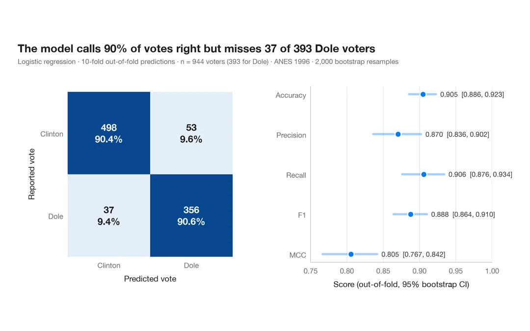
Confusion matrix with metrics
How well a logistic regression predicts who voted Dole in 1996 — out-of-fold confusion matrix with counts and row shares, and bootstrap intervals for the headline metrics.
yardstick::conf_mat() + autoplot()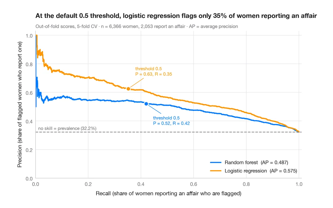
Precision–recall curves
Out-of-fold precision–recall curves for two classifiers predicting which married women report an affair, with average precision and the no-skill baseline.
yardstick::pr_curve() + autoplot()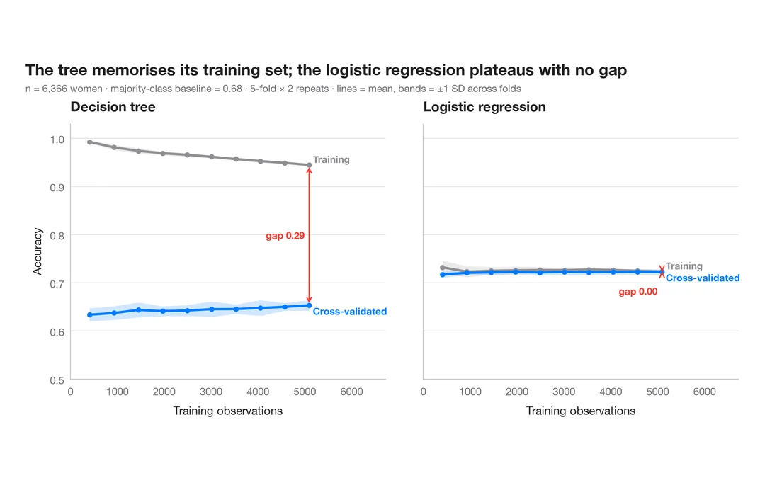
Learning curve
Training and cross-validated accuracy as the training set grows, for two models predicting which married women report an affair.
caret::learning_curve_dat() + ggplot()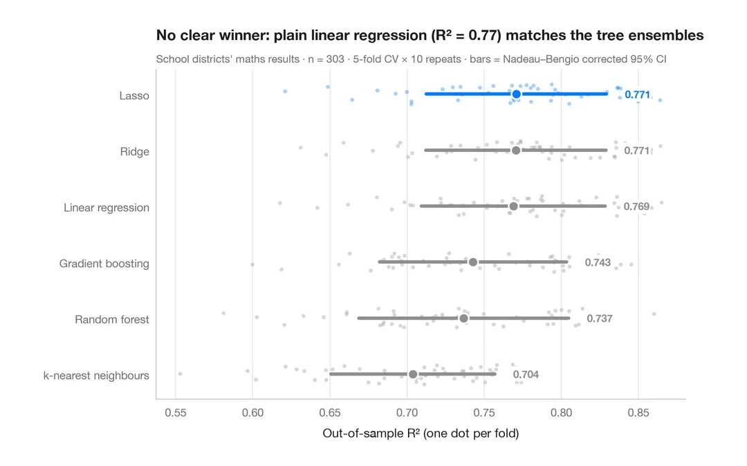
Cross-validated model comparison
Fold-by-fold R² of six models predicting California school districts' maths results, with means and corrected 95% intervals.
caret::resamples() + bwplot() / tune::autoplot()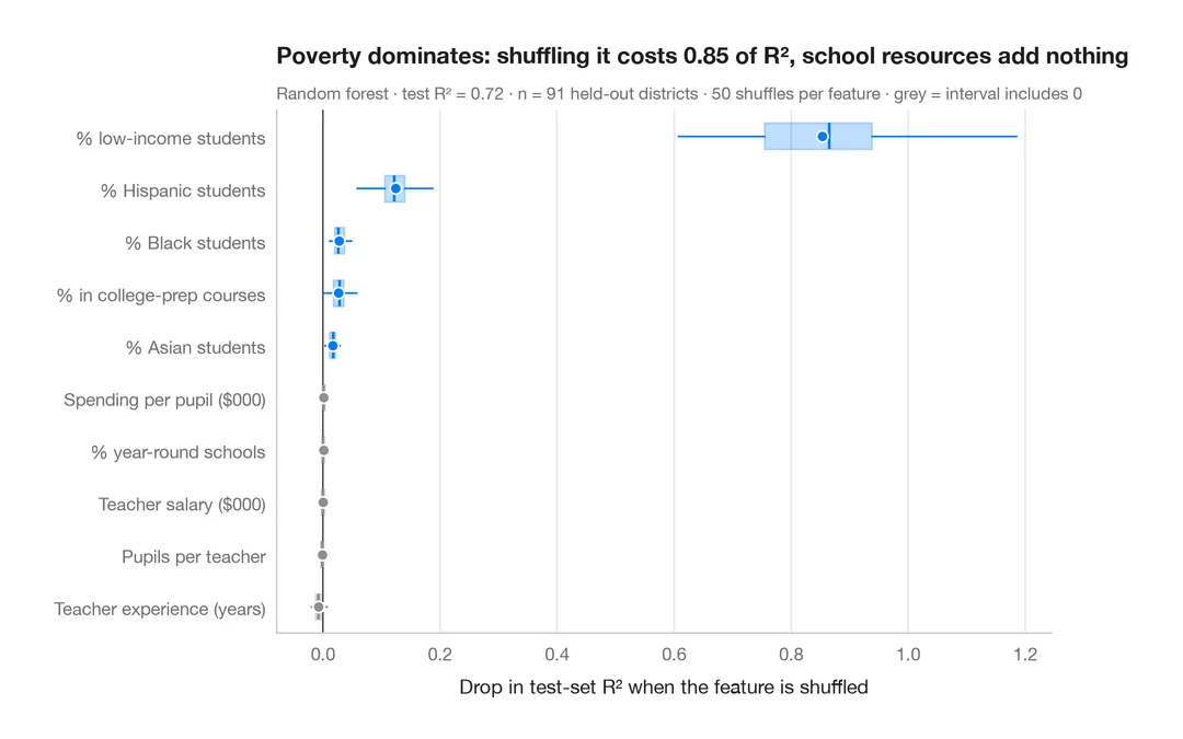
Permutation importance
Which district characteristics a random forest relies on to predict maths results — drop in test-set R² when each one is shuffled.
vip::vip(method = "permute")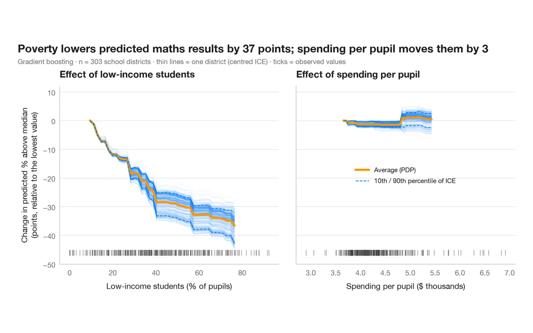
Partial dependence with ICE curves
How predicted maths results change with poverty and with spending per pupil — the average (PDP) over one curve per school district (ICE).
pdp::partial(ice = TRUE) + autoplot() / iml::FeatureEffectAdvanced: SHAP explanations
Shapley values split every prediction into additive feature contributions — globally, feature by feature, and for a single case.
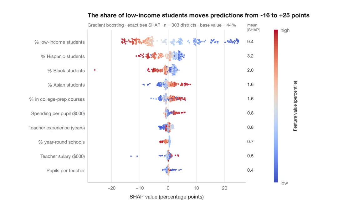
SHAP summary (beeswarm)
Every school district's SHAP value for every characteristic, coloured by the characteristic's value, with mean |SHAP| importance.
shapviz::sv_importance(kind = "beeswarm")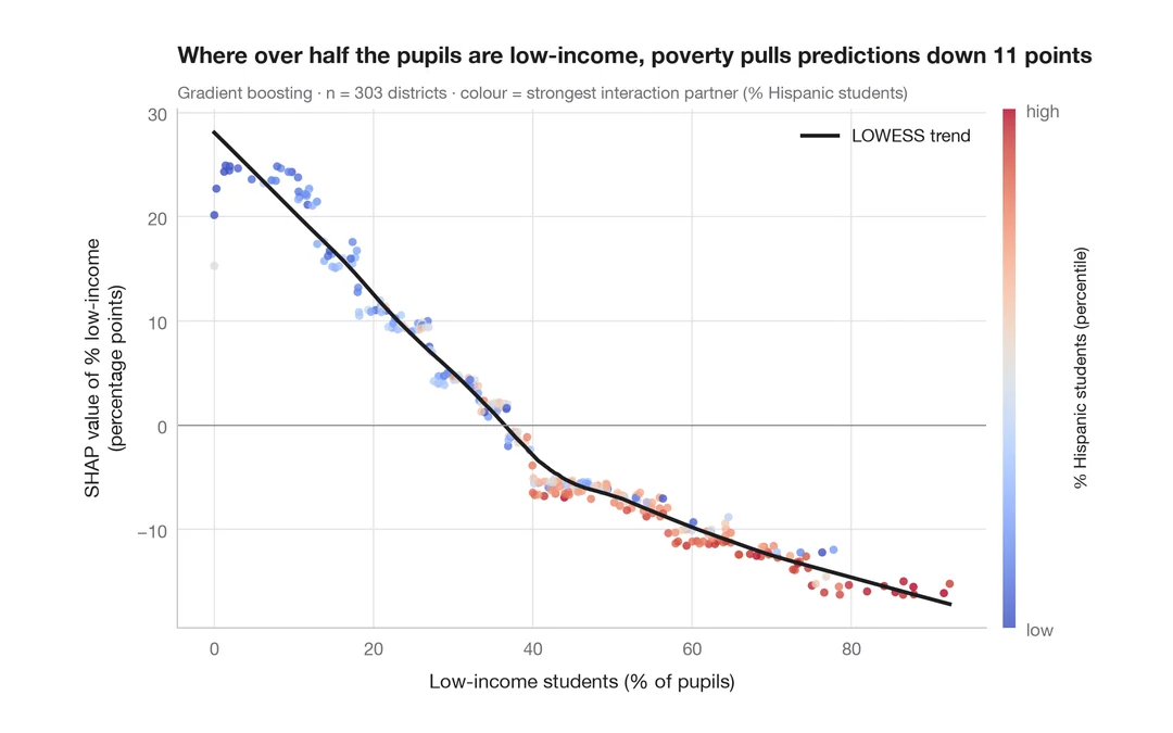
SHAP dependence plot
How the share of low-income students feeds into each district's predicted maths results, coloured by its strongest interaction partner, with a smooth trend.
shapviz::sv_dependence()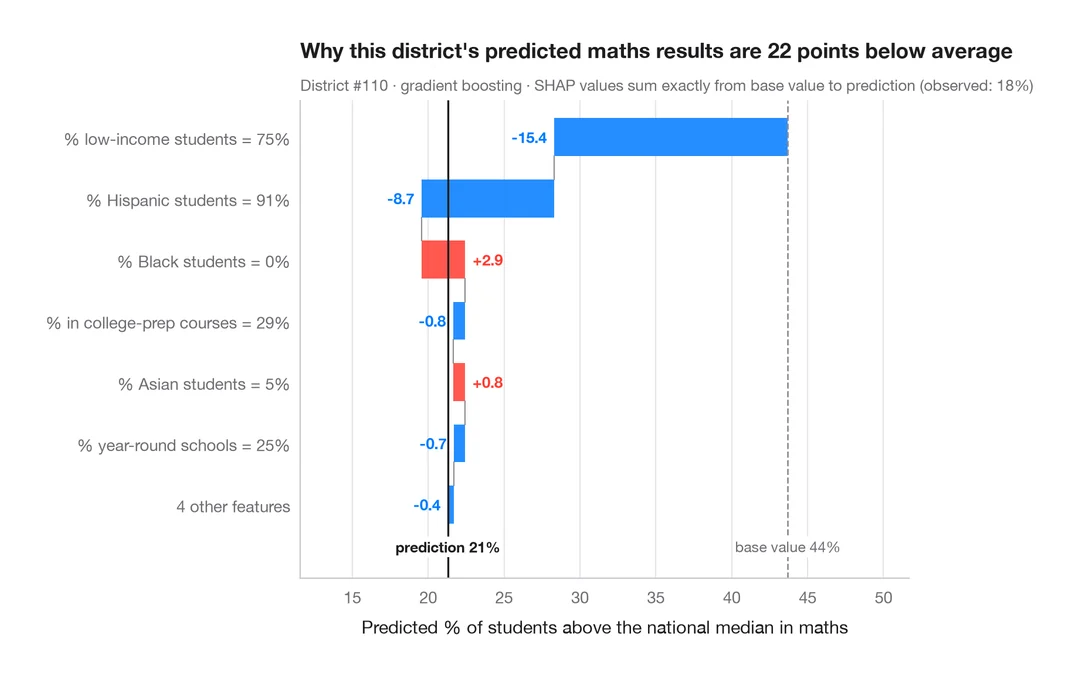
SHAP waterfall for one prediction
How each characteristic moves one struggling school district's predicted maths results from the average to the model's output.
shapviz::sv_waterfall()Spatial data
Is a value higher where its neighbours' values are higher? Spatial weights, global and local spatial autocorrelation, and how far clusters reach — on Guerry's 1830s France.
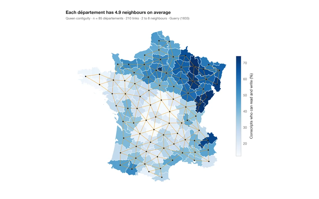
Choropleth with spatial weights
A map of one variable with the neighbour network drawn on top — the structure every spatial statistic relies on.
spdep::poly2nb() + plot(nb, coords)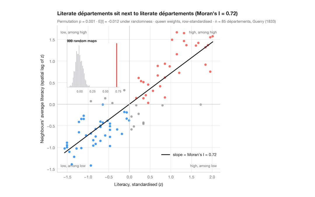
Moran scatterplot (global autocorrelation)
Each area against the average of its neighbours, with Moran's I, its permutation test and the reference distribution.
spdep::moran.plot() + spdep::moran.mc()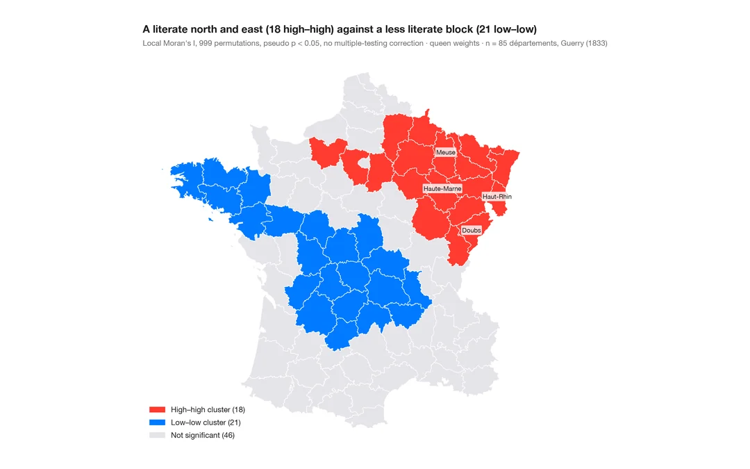
LISA cluster map (local autocorrelation)
Where the clusters and spatial outliers are — local Moran's I for each area, mapped with its permutation significance.
spdep::localmoran_perm() / rgeoda::local_moran()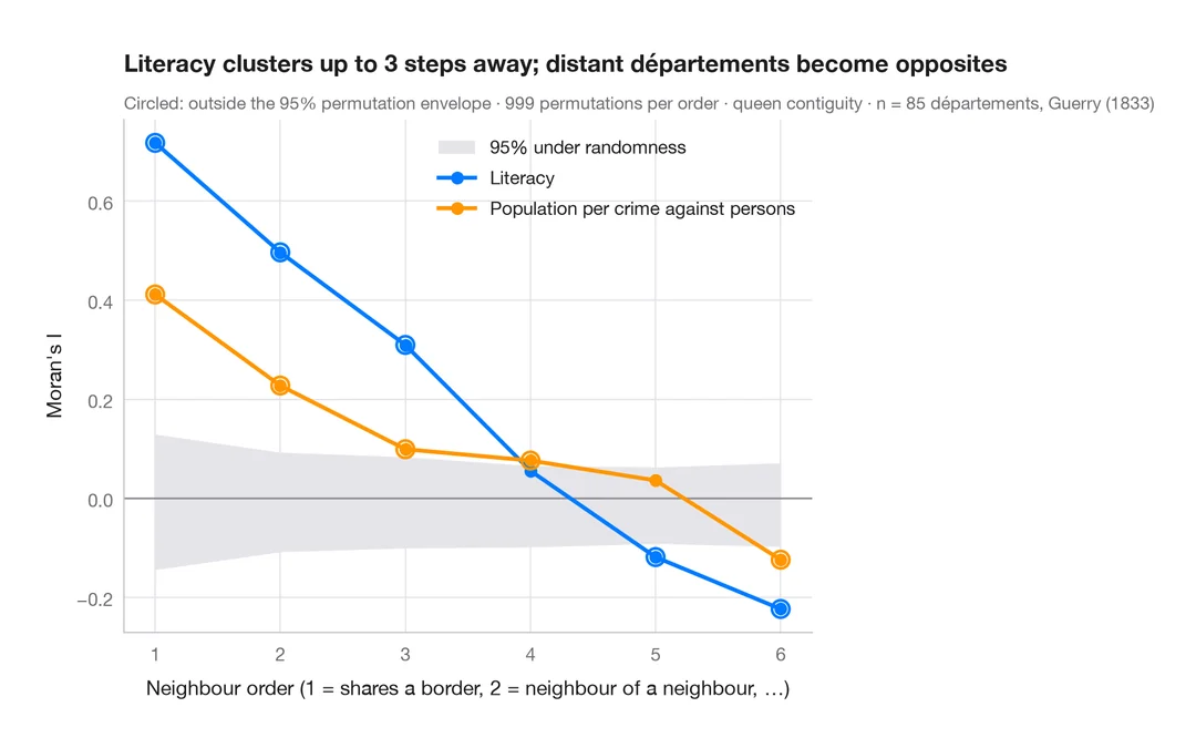
Spatial correlogram
Moran's I at increasing neighbour orders, with a permutation envelope — how far spatial clustering reaches.
spdep::sp.correlogram(method = "I")Distributions
See the shape of your data: histograms, densities, ridgelines, ECDFs and Q–Q plots.
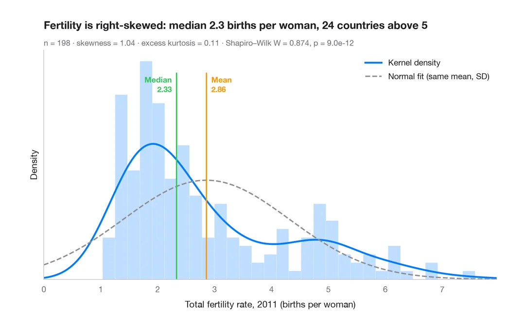
Histogram with density
Histogram, kernel density and fitted normal curve, with shape statistics.
ggplot2::geom_histogram() + geom_density()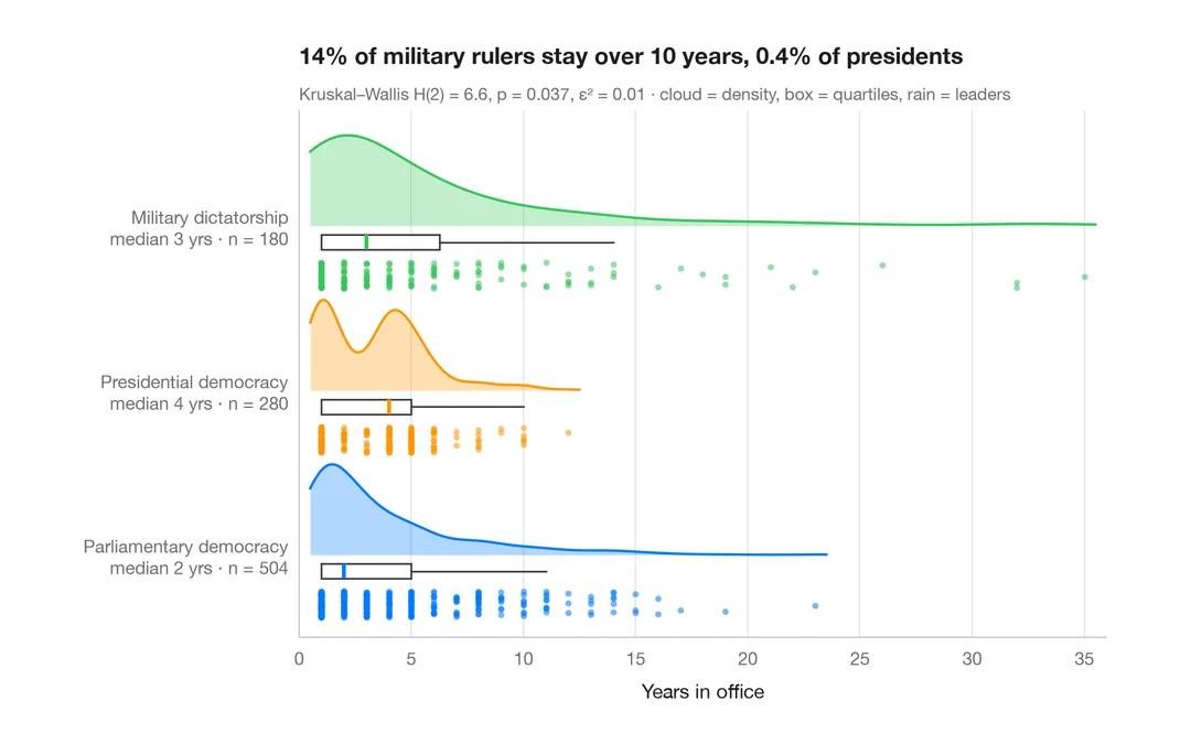
Raincloud plot
Half violin, box plot and raw points per group, drawn horizontally.
ggdist::stat_halfeye() / ggrain::geom_rain()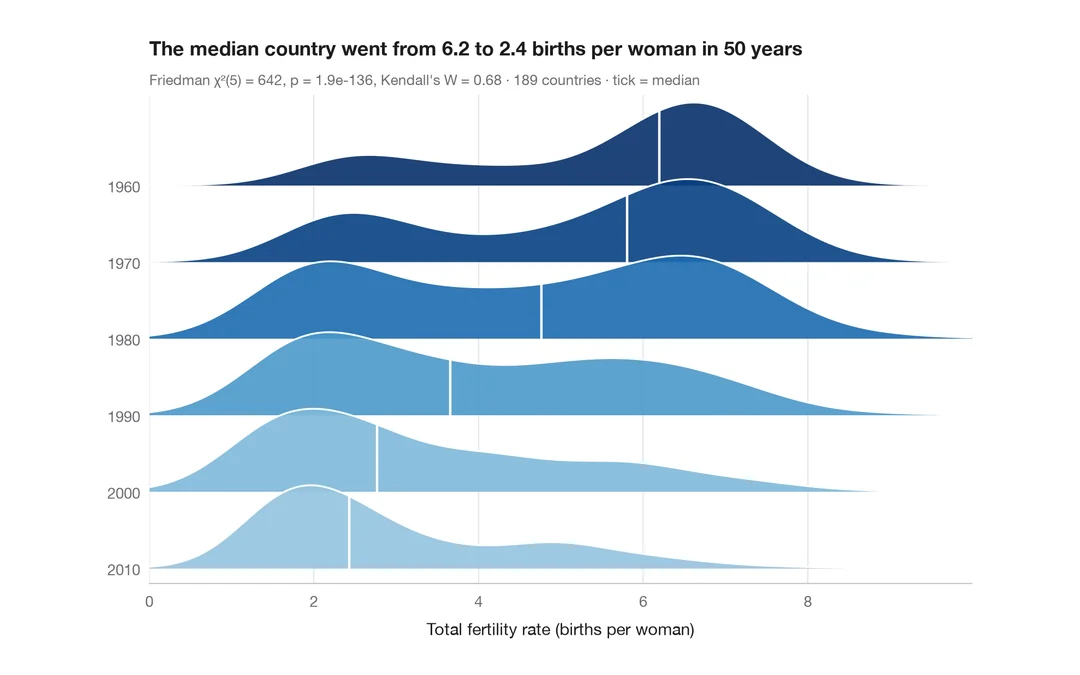
Ridgeline plot
Overlapping density curves to compare one distribution across many groups.
ggridges::geom_density_ridges()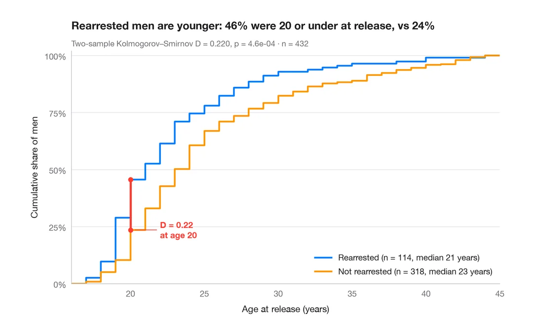
ECDF comparison
Empirical cumulative distributions of two groups, with the Kolmogorov–Smirnov gap.
ggplot2::stat_ecdf()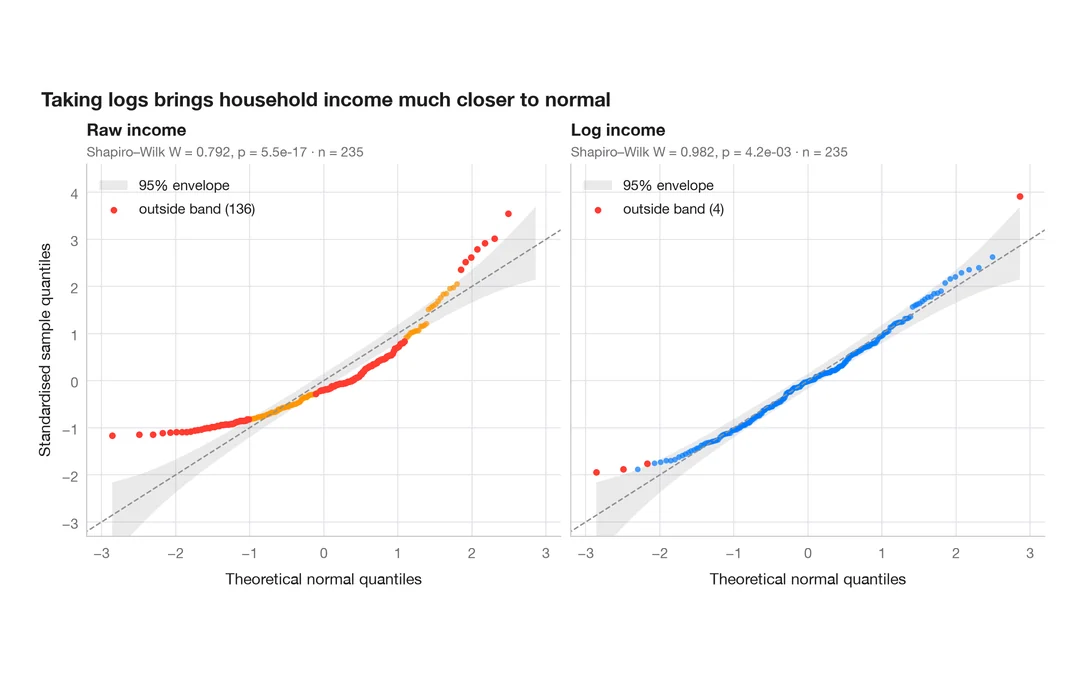
Q–Q plot with confidence band
Normal quantile–quantile plots with a 95% envelope, for a raw and a logged variable.
qqplotr::stat_qq_band()Group comparisons
Compare groups with the test, effect size and p-values on the chart — the ggstatsplot way.
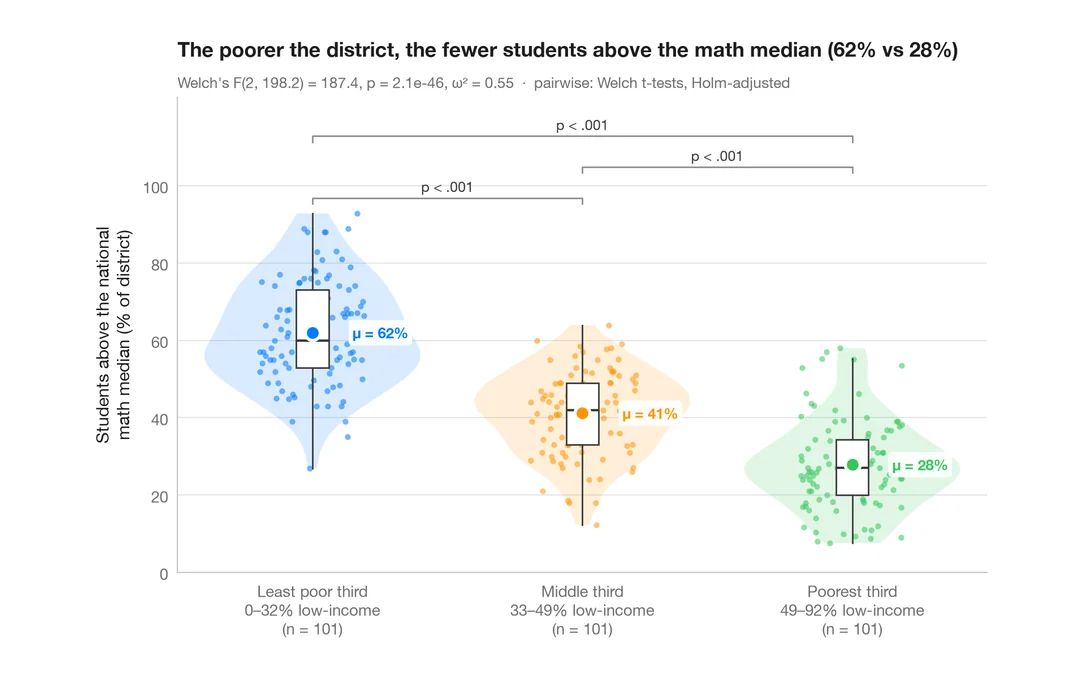
Between-groups comparison
Violin + box + points with Welch's ANOVA, effect size and pairwise tests.
ggstatsplot::ggbetweenstats()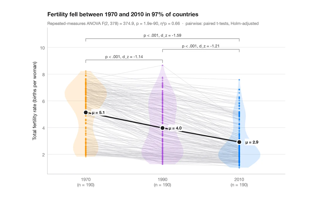
Within-subjects comparison
Repeated measures with one line per subject, means, rm-ANOVA and paired tests.
ggstatsplot::ggwithinstats()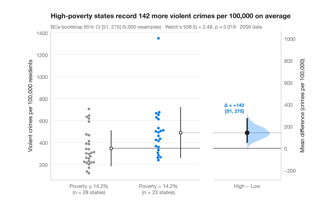
Estimation plot
Raw data of two groups plus the mean difference and its bootstrap 95% CI.
dabestr::dabest() + plot()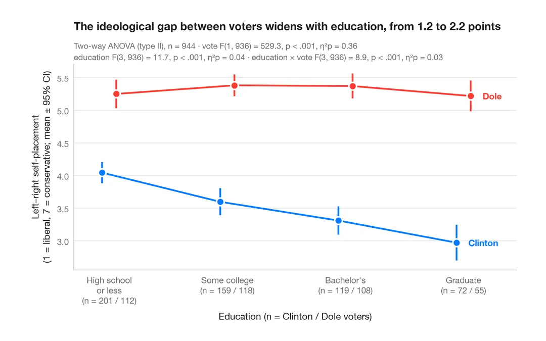
Interaction plot
Group means with 95% confidence intervals for two factors, with a two-way ANOVA.
ggpubr::ggline(add = "mean_ci") / ggstats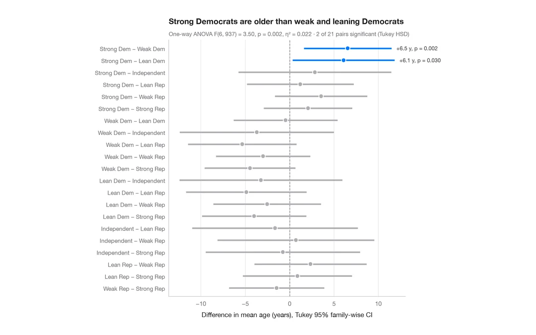
Tukey HSD intervals
Simultaneous 95% confidence intervals for every pairwise difference in means.
TukeyHSD() + plot()Proportions & surveys
Proportions, cross-tabs and Likert scales, in the spirit of ggstats::gglikert and stat_prop.
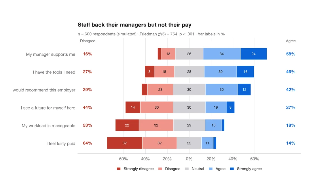
Diverging Likert chart
Five-point Likert items as diverging stacked bars centred on the neutral answer.
ggstats::gglikert()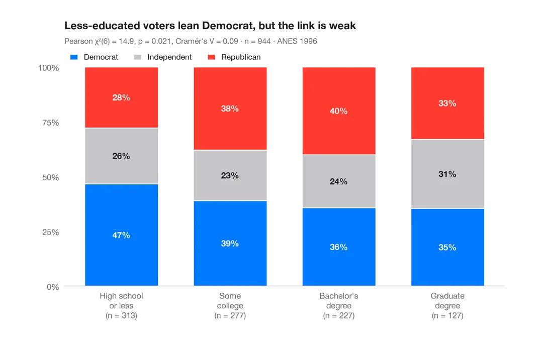
Stacked proportions by group
100% stacked bars with percentage labels, n per bar, chi-squared test and Cramér's V.
ggstatsplot::ggbarstats()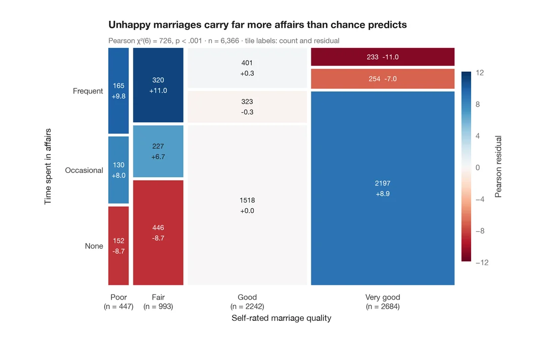
Mosaic plot with Pearson residuals
Tile areas proportional to cell counts, shaded by Pearson residuals from independence.
vcd::mosaic(shade = TRUE)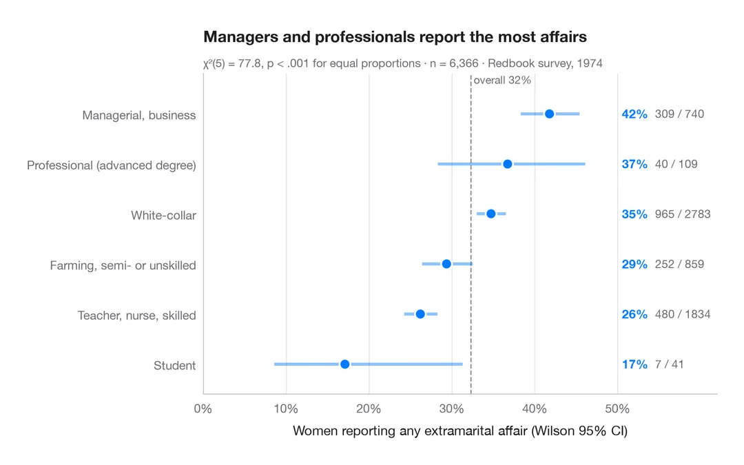
Proportions with confidence intervals
A sorted dot plot of group proportions with Wilson 95% confidence intervals.
ggstats::stat_prop() + geom_errorbar()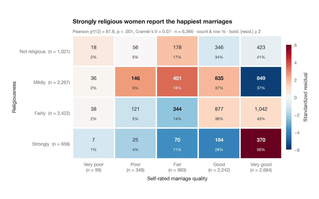
Cross-table with standardized residuals
A contingency table as a heatmap, coloured by standardized residuals from independence.
ggstats::ggtable() / stat_cross()Correlation & association
Correlation matrices, scatterplots with statistics and pairwise relationships.
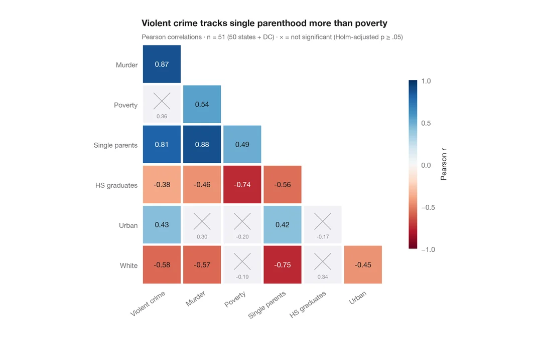
Correlation matrix
Lower-triangle Pearson correlation heatmap; non-significant cells (Holm) are crossed out.
ggstatsplot::ggcorrmat()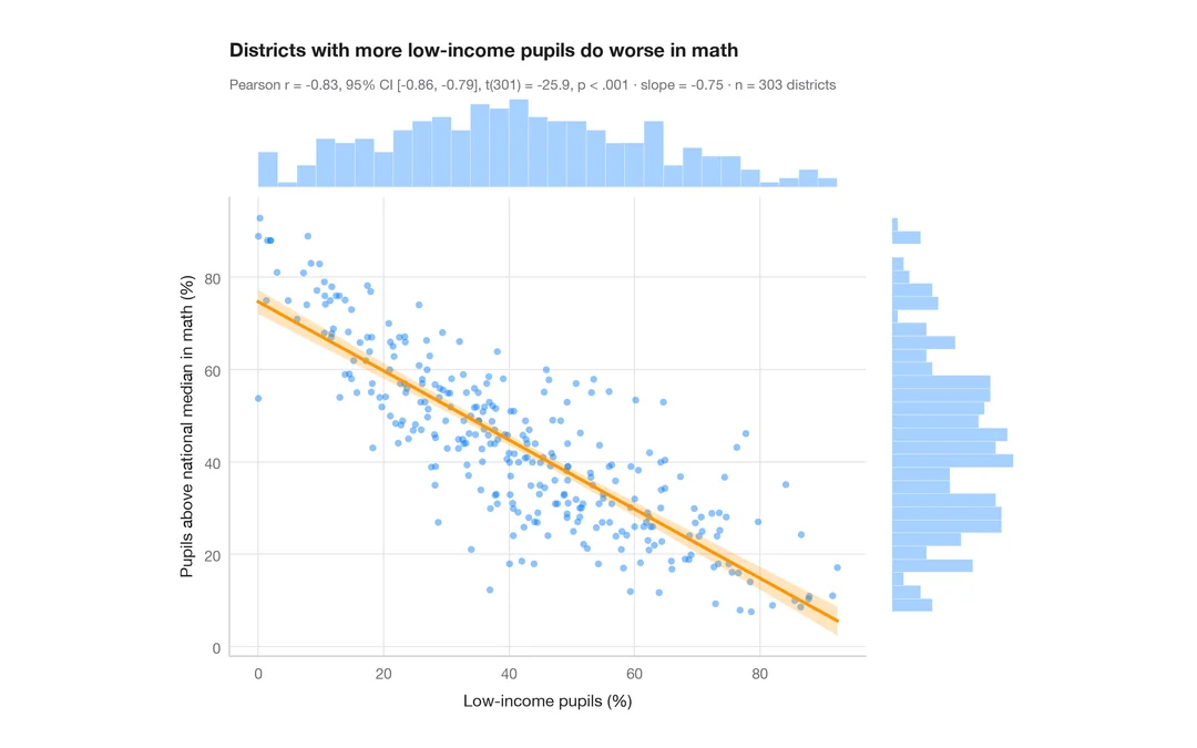
Scatterplot with statistics
Low-income pupils vs math results in 303 California districts — scatter, OLS line with 95% band, marginal histograms and Pearson's r.
ggstatsplot::ggscatterstats()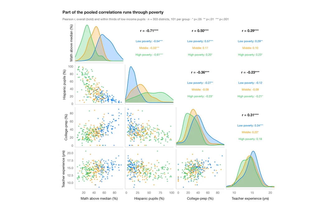
Pairs plot with correlations
Scatter matrix of four school-district variables, with group KDEs on the diagonal and pooled vs within-group correlations above it.
GGally::ggpairs()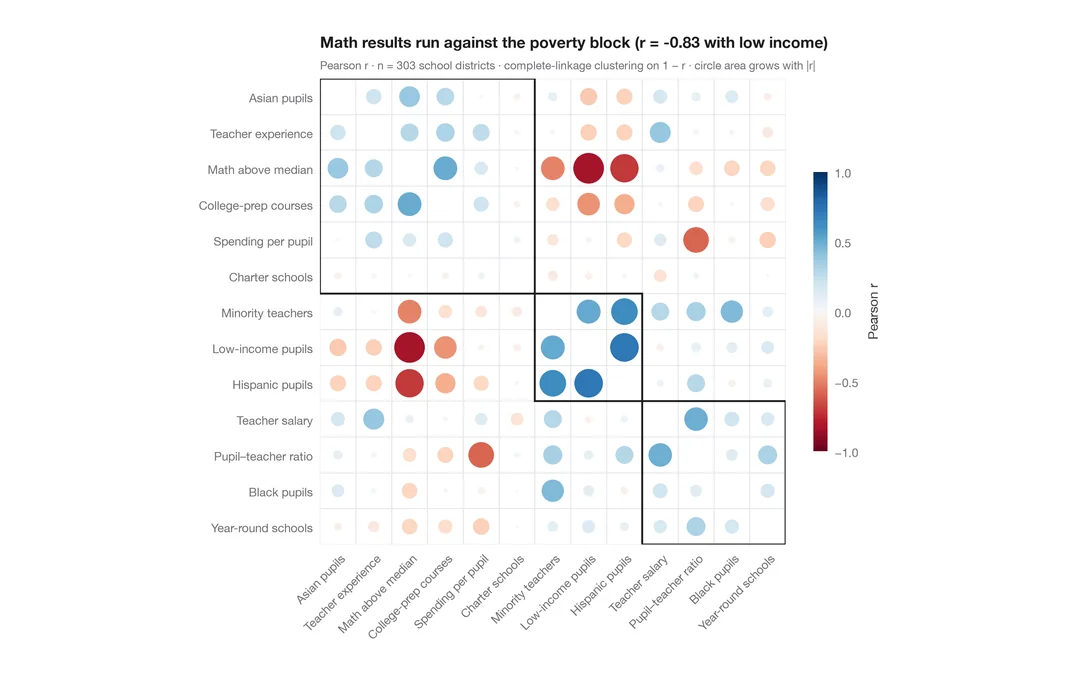
Correlogram with clustering
Corrplot-style circles sized and coloured by r for 13 school-district indicators, ordered by hierarchical clustering.
corrplot::corrplot(order = "hclust", addrect = 3)Regression models
Coefficient plots, odds ratios, model comparison and marginal effects — ggcoef_model for Python.
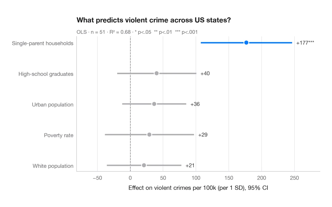
Coefficient plot
Regression estimates with 95% confidence intervals, one row per term.
ggstats::ggcoef_model()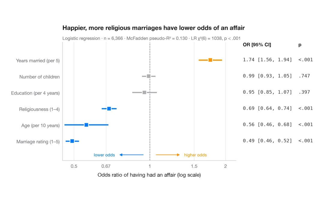
Odds-ratio forest plot
Logistic regression odds ratios on a log scale, with a table of OR [95% CI] alongside.
ggstats::ggcoef_model(exponentiate = TRUE)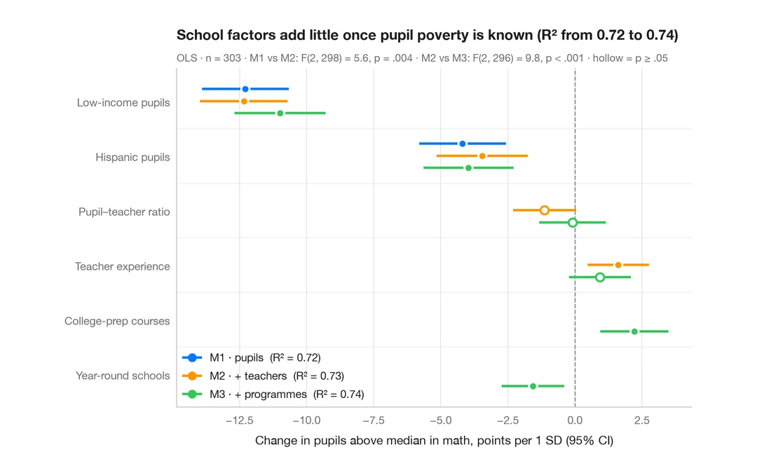
Comparing nested models
Coefficients of three nested regressions of district math results side by side, to see how estimates shift as blocks are added.
ggstats::ggcoef_compare()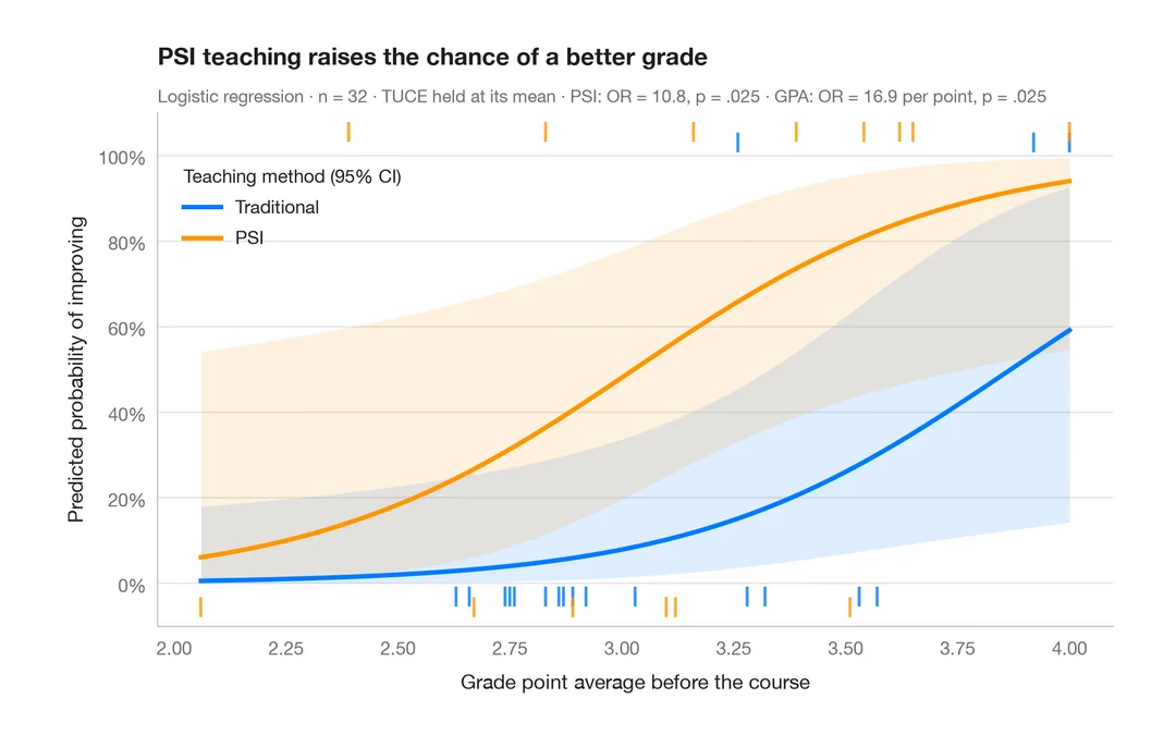
Predicted probabilities
Model-based probability curves with 95% CI ribbons across a predictor, by group.
ggeffects::ggpredict() / marginaleffects::plot_predictions()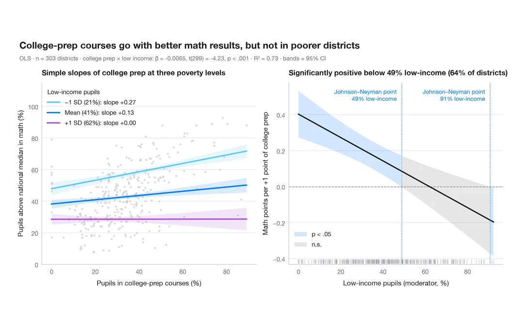
Interaction effects
Simple slopes at mean ± 1 SD and a Johnson–Neyman plot for college-prep courses and math results, moderated by pupil poverty.
interactions::interact_plot() / interactions::johnson_neyman()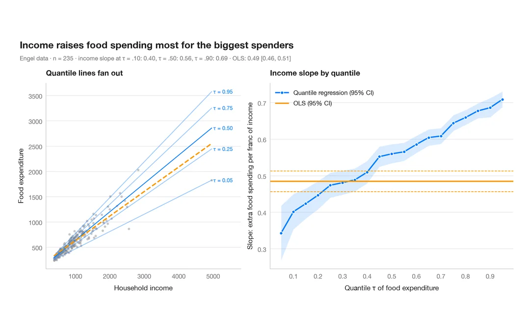
Quantile regression process
How a slope changes across the conditional distribution, against the single OLS estimate.
quantreg::plot(summary(rq(tau = 1:19 / 20)))Model diagnostics
Residuals, leverage, calibration and ROC curves: check before you trust a model.
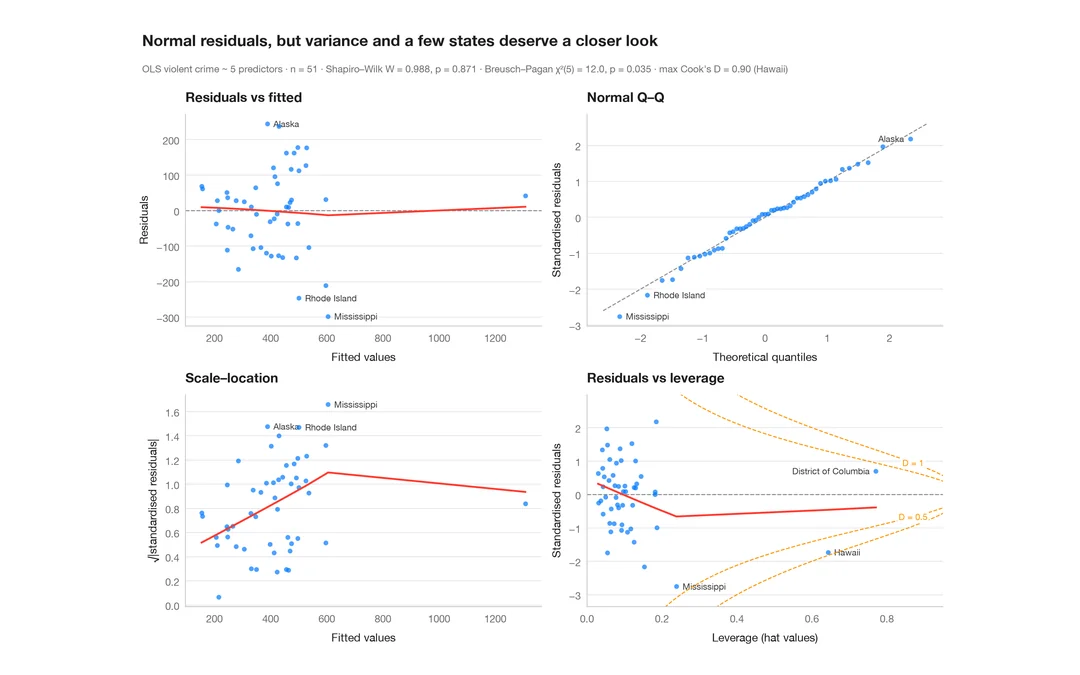
Residual diagnostics
The classic 2 × 2 panel for a linear model — linearity, normality, variance, leverage.
plot(lm) / performance::check_model()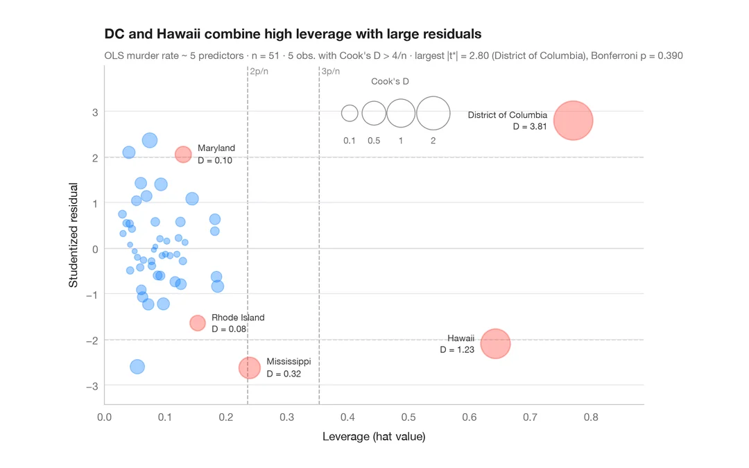
Influence plot
Studentized residuals vs leverage, with bubbles sized by Cook's distance.
car::influencePlot()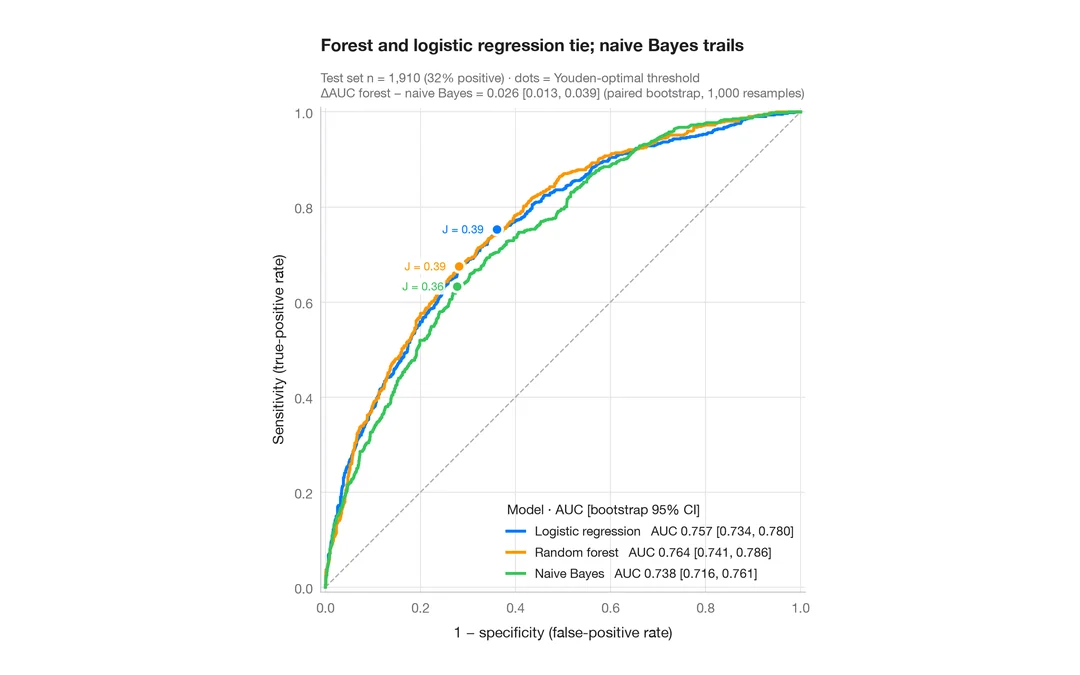
ROC curves
Three classifiers compared by ROC curve, AUC with bootstrap 95% CI and Youden point.
pROC::ggroc() / pROC::ci.auc()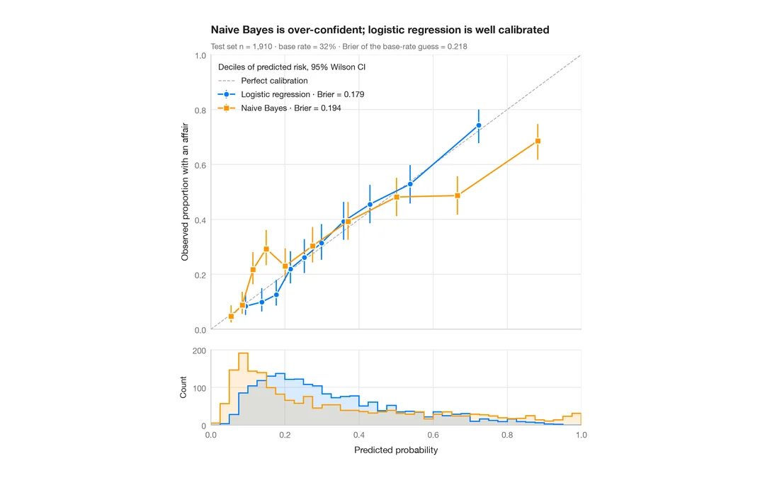
Calibration plot
Predicted vs observed risk per decile, with Wilson CIs, prediction histograms and Brier score.
rms::calibrate() / probably::cal_plot_breaks()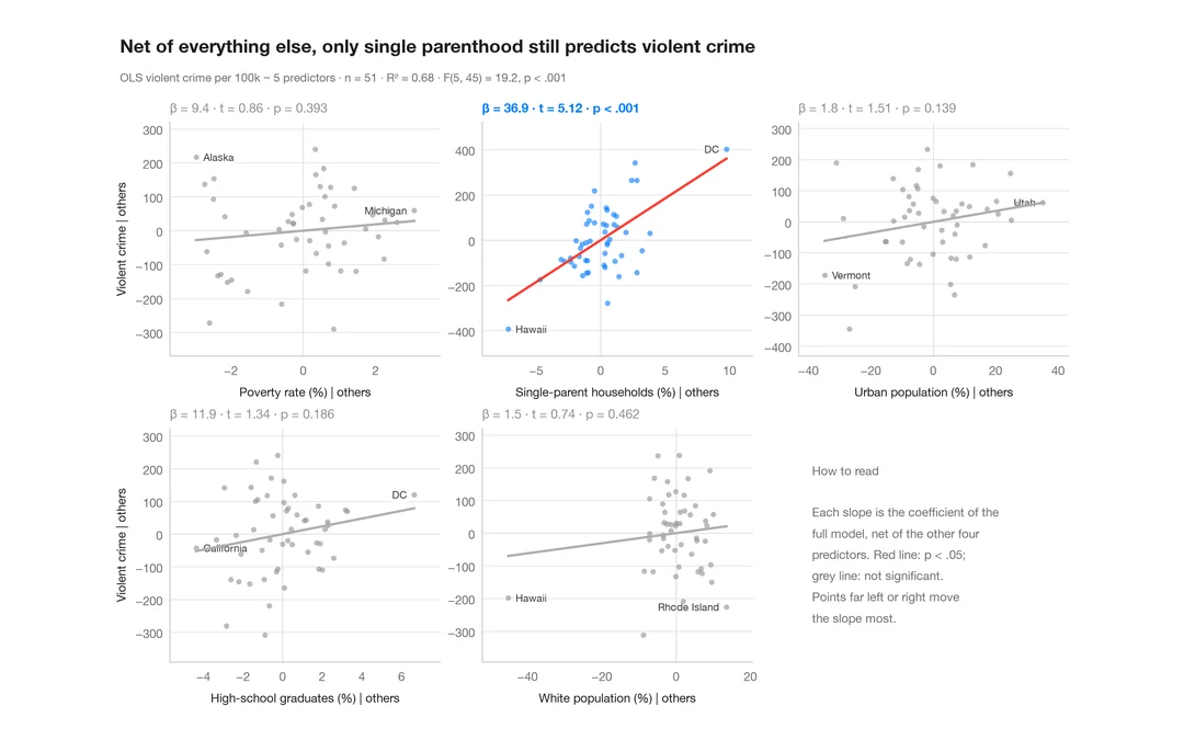
Added-variable plots
One partial-regression panel per predictor; each fitted slope equals its coefficient.
car::avPlots()Survival analysis
Kaplan–Meier curves with risk tables, cumulative hazards and Cox model hazard ratios.
Kaplan–Meier curves
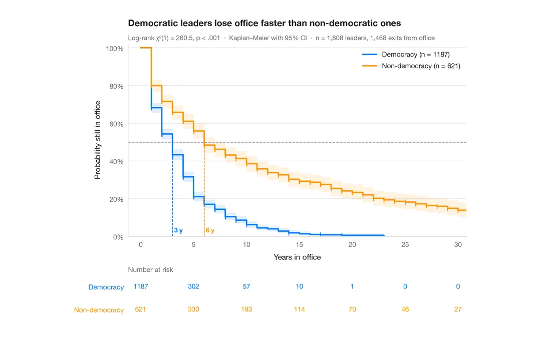
How long political leaders stay in office, democracies vs non-democracies — survival curves with confidence bands, censoring marks, log-rank test and risk table.
survminer::ggsurvplot(risk.table = TRUE)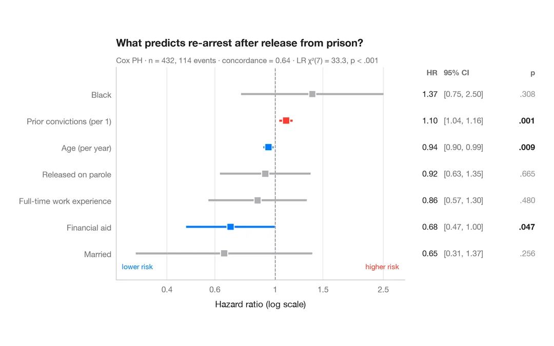
Cox hazard ratios
Forest plot of a Cox proportional hazards model with HR, 95% CI and p-values.
survminer::ggforest()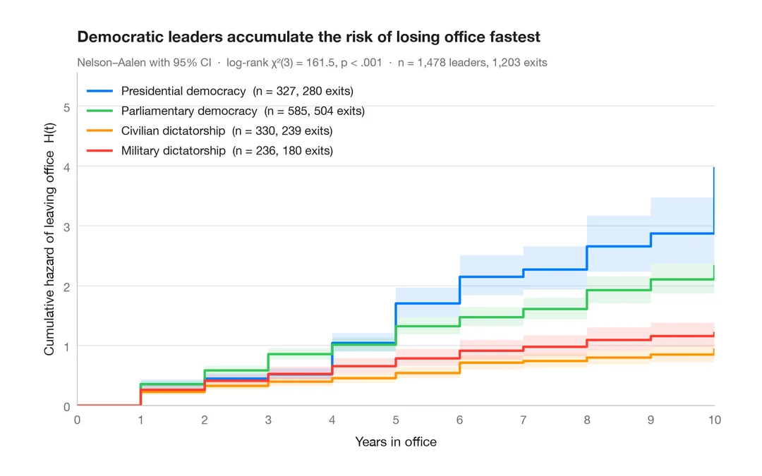
Cumulative hazard
Nelson–Aalen cumulative hazard of leaving office, with 95% bands, for four political regimes.
survminer::ggsurvplot(fun = "cumhaz")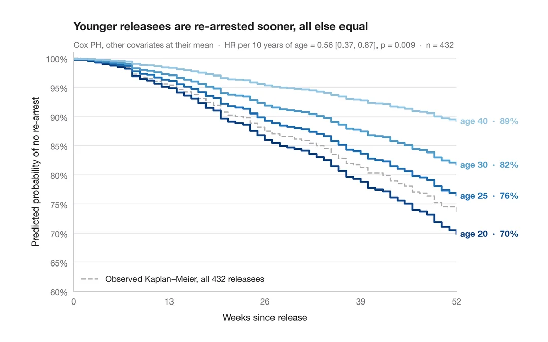
Adjusted survival curves
Cox model–predicted survival for several ages, other covariates held at their mean.
survminer::ggadjustedcurves()Time series
Decomposition, autocorrelation, forecasts with prediction intervals and change over time.
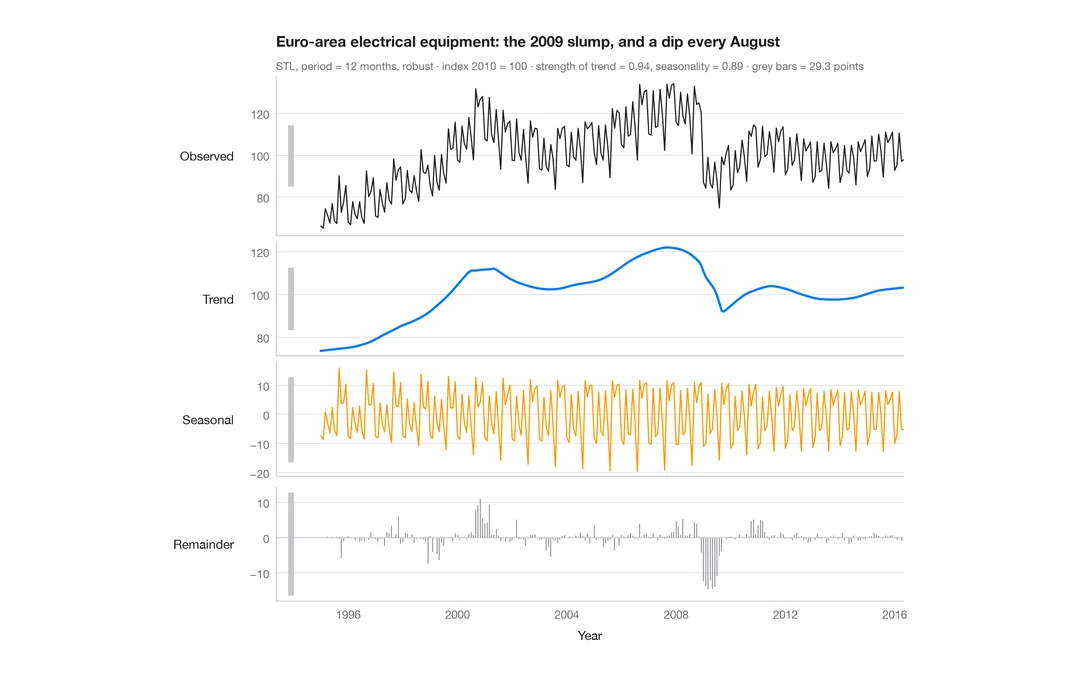
STL decomposition
A monthly industrial turnover series split into trend, seasonal and remainder components in stacked panels.
feasts::STL() + autoplot()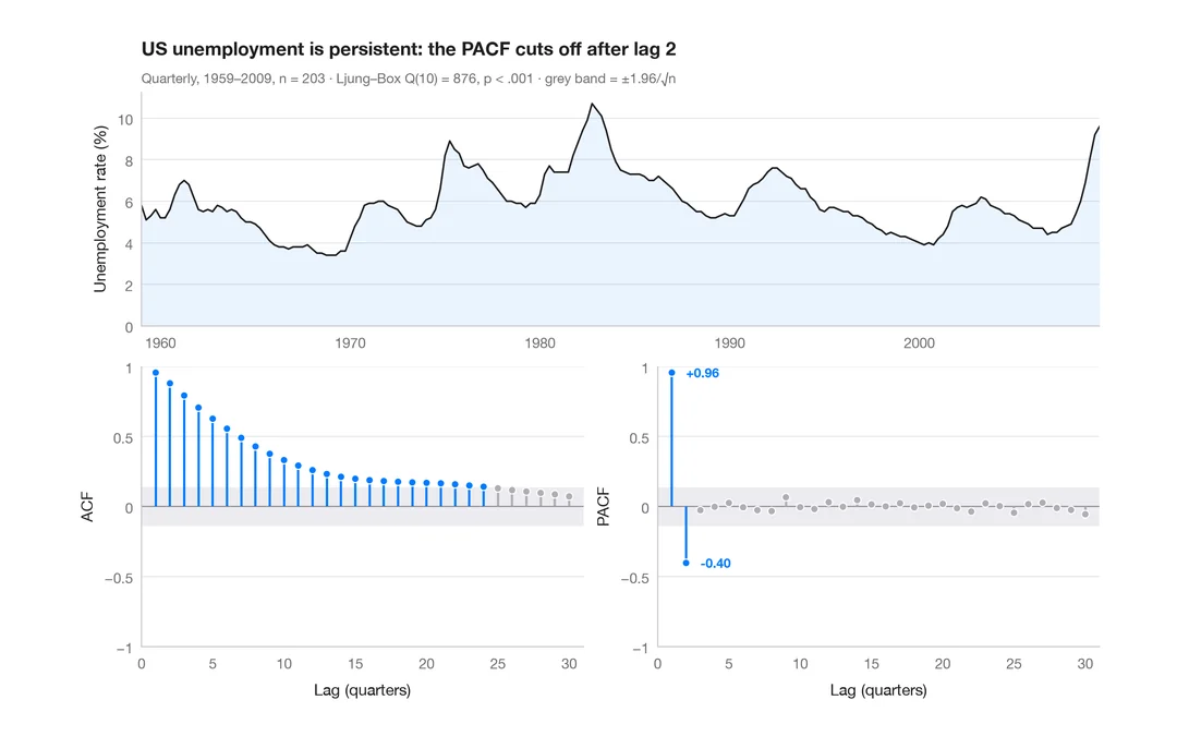
ACF and PACF
Autocorrelation and partial autocorrelation of US quarterly unemployment, as lollipops with 95% significance bands.
forecast::ggtsdisplay()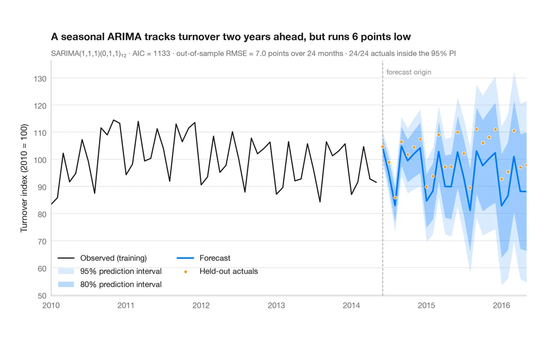
SARIMA forecast
Seasonal ARIMA forecast of industrial turnover with 80% and 95% prediction intervals against held-out data.
forecast::autoplot(forecast())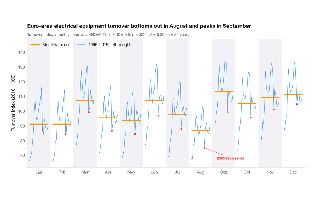
Seasonal subseries plot
Each calendar month's industrial turnover across the years, with the monthly mean as a reference.
feasts::gg_subseries()Multivariate & clustering
PCA biplots, scree plots, clustering and heatmaps for high-dimensional data.
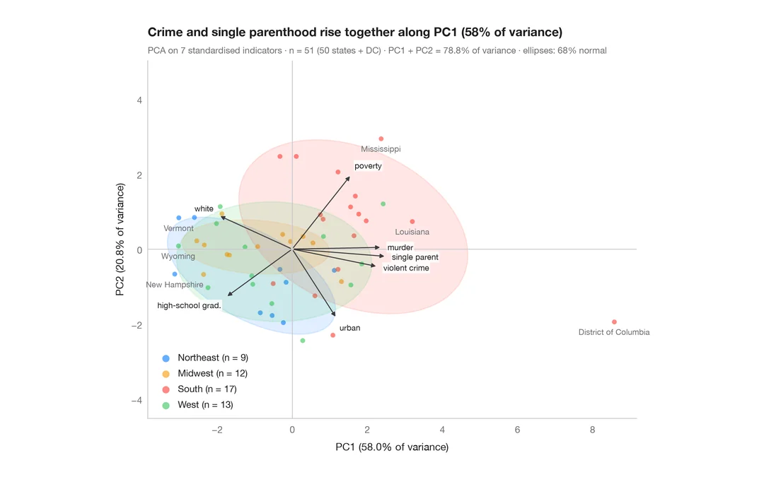
PCA biplot
US states and their social indicators on the first two principal components.
factoextra::fviz_pca_biplot()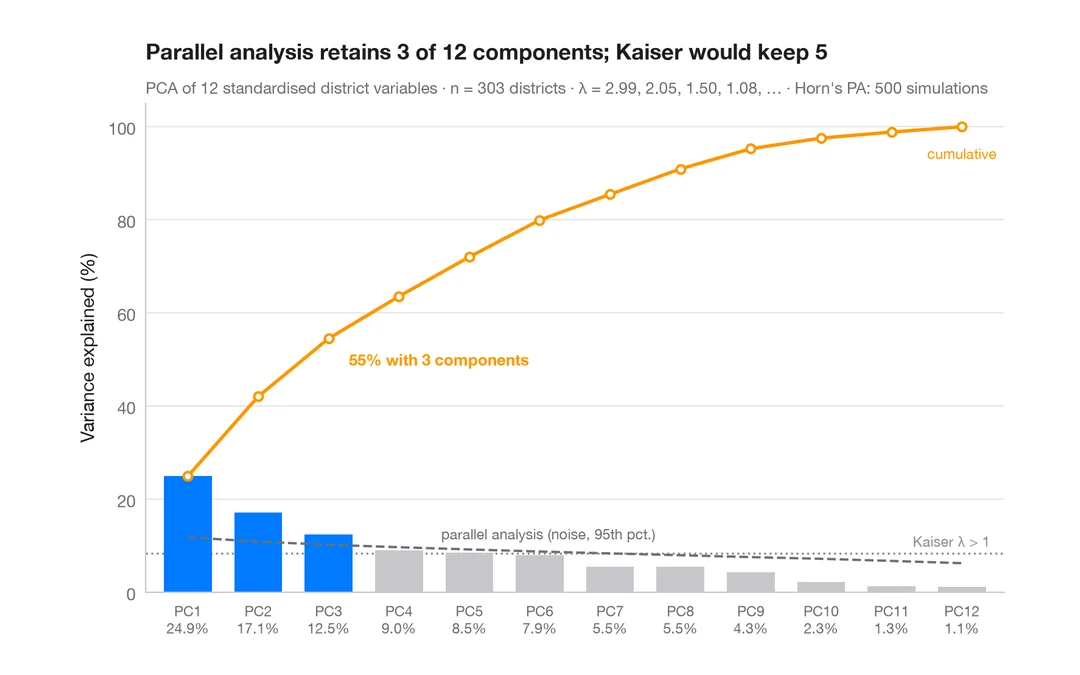
Scree plot
How many dimensions describe 303 California school districts? Variance per component and a parallel-analysis cut-off.
factoextra::fviz_eig()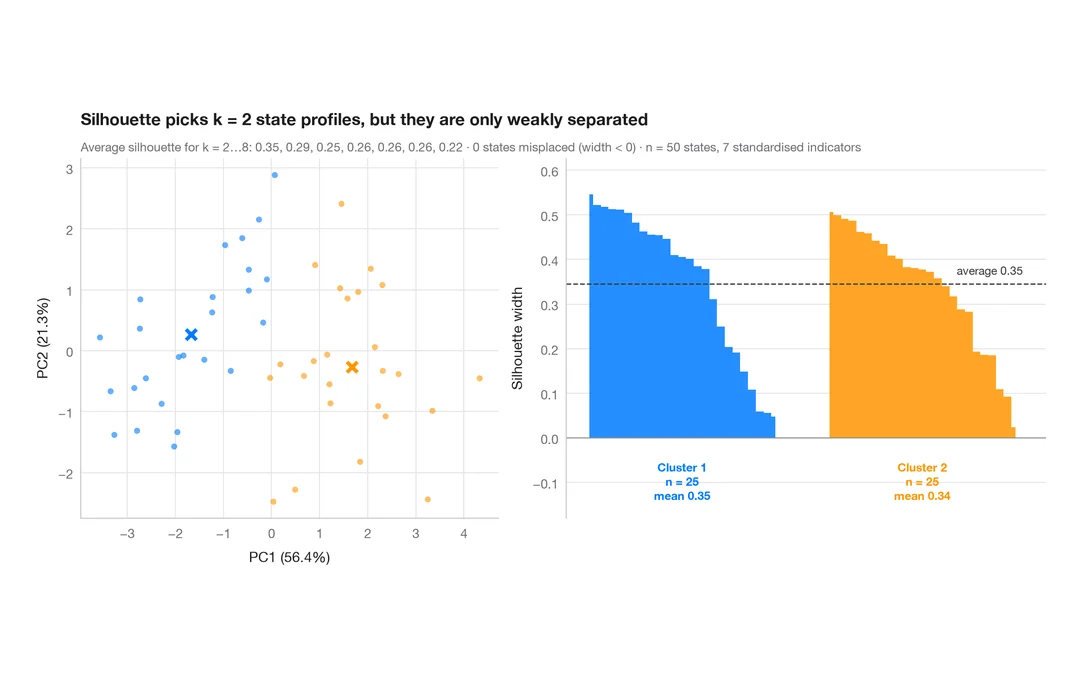
Silhouette plot for k-means
Do US states fall into distinct social profiles? k-means clusters next to their silhouette widths.
factoextra::fviz_silhouette()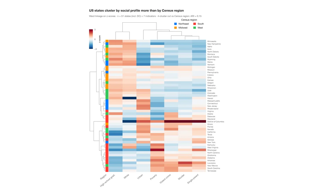
Clustered heatmap
Z-scored heatmap of US states' social indicators, with row and column dendrograms and a Census-region colour bar.
pheatmap::pheatmap() / ComplexHeatmap::Heatmap()Inference & uncertainty
Bootstrap, confidence intervals, power, agreement and meta-analysis forest plots.
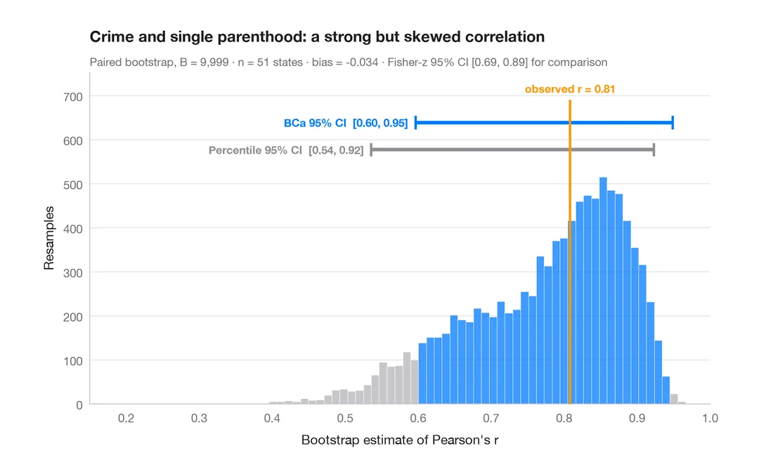
Bootstrap distribution
Resampled correlation with percentile and BCa 95% confidence intervals.
boot::boot() + boot::boot.ci()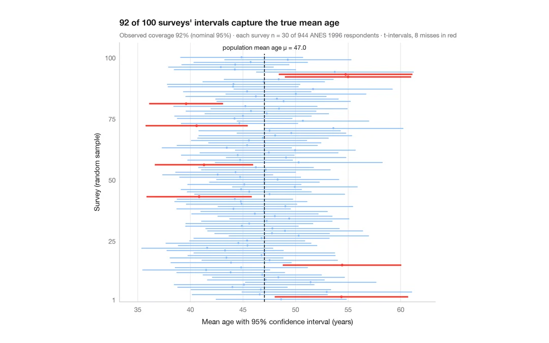
What a 95% confidence interval means
100 surveys of 30 people drawn from 944 ANES respondents; the 95% CIs for mean age that miss the true value are in red.
teaching classic (e.g. TeachingDemos::ci.examp())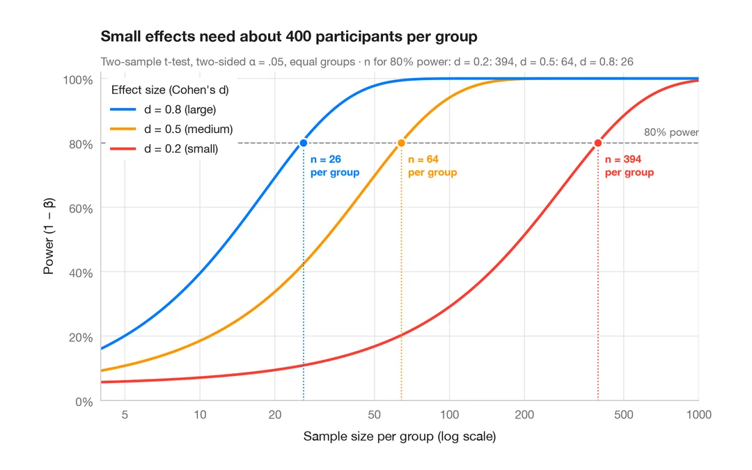
Power curve
Power of a two-sample t-test against sample size for small, medium and large effects.
pwr::pwr.t.test() + plot()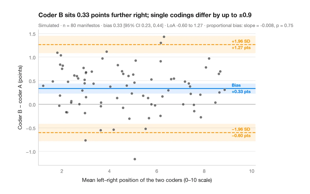
Bland–Altman plot
Do two coders place party manifestos on the left–right scale the same way? Bias and 95% limits of agreement.
BlandAltmanLeh::bland.altman.plot() / blandr::blandr.draw()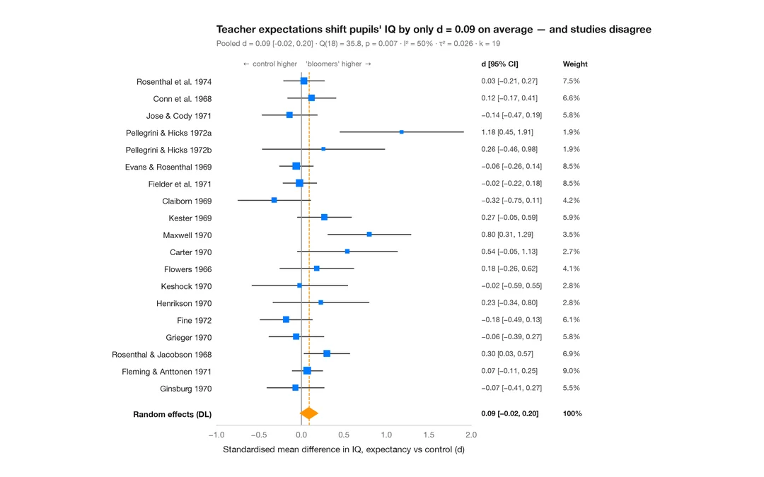
Meta-analysis forest plot
Do teacher expectations raise pupils' IQ? 19 "Pygmalion" experiments, a random-effects pooled diamond and heterogeneity statistics.
meta::forest() / metafor::forest()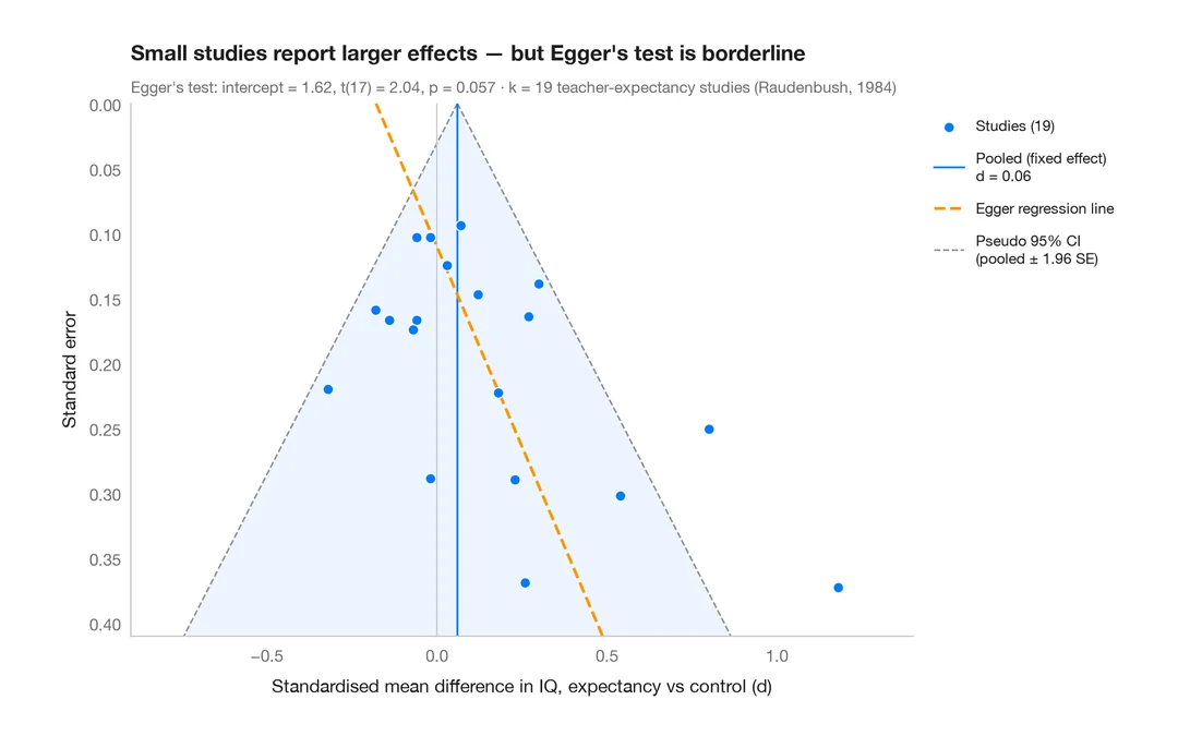
Funnel plot
Are small "Pygmalion" studies more optimistic? 19 teacher-expectancy effects against their standard error, with a pseudo 95% funnel and Egger's test.
metafor::funnel() + metafor::regtest()How to cite
PyStatlas is created and maintained by Thierry Warin. If it helped your work, please cite it.
Warin, T. (2026). PyStatlas: A Python Gallery of Statistical Graphics for the Social Sciences. https://warint.github.io/pystatlas/
@misc{warin2026statlas,
  author       = {Warin, Thierry},
  title        = {PyStatlas: A Python Gallery of Statistical Graphics for the Social Sciences},
  year         = {2026},
  howpublished = {\url{https://warint.github.io/pystatlas/}},
  note         = {Source code: https://github.com/warint/pystatlas}
}