Quantile regression process
How a slope changes across the conditional distribution, against the single OLS estimate.
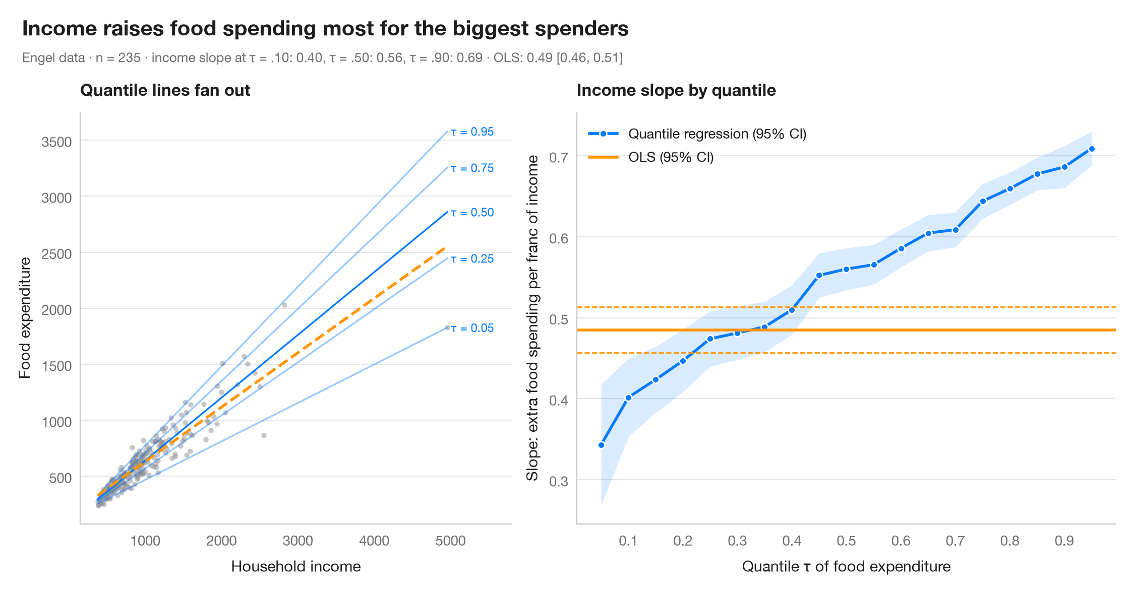
OLS estimates one slope: the effect on the conditional mean. Quantile regression estimates a slope for every conditional quantile τ, so you can see whether a predictor stretches the distribution rather than just shifting it. The dark line is the quantile-regression coefficient for τ = 0.05 … 0.95, with its 95% band; the orange line and dashed lines are the OLS estimate and its 95% CI, constant by construction. The left panel shows the data with a few of the fitted quantile lines.
Data are Engel's (1857) household budget survey of 235 Belgian working-class
families, bundled with statsmodels (sm.datasets.engel). Models are fitted
with smf.quantreg().fit(q=τ) and smf.ols().
import matplotlib.pyplot as plt
import numpy as np
import statsmodels.api as sm
import statsmodels.formula.api as smf

# Data: Engel food expenditure vs household income (Belgian francs)
df = sm.datasets.engel.load_pandas().data
quantiles = np.arange(0.05, 0.96, 0.05)

# Fit one quantile regression per τ and keep slope + 95% CI
rows = []
for q in quantiles:
    fit = smf.quantreg("foodexp ~ income", df).fit(q=q)
    lo, hi = fit.conf_int().loc["income"]
    rows.append((q, fit.params["Intercept"], fit.params["income"], lo, hi))
qr = np.array(rows)
ols = smf.ols("foodexp ~ income", df).fit()
ols_lo, ols_hi = ols.conf_int().loc["income"]

fig, (ax1, ax2) = plt.subplots(1, 2, figsize=(11, 5), gridspec_kw=dict(width_ratios=[1, 1.25]))

# Left: data with selected quantile lines and the OLS line
ax1.scatter(df.income, df.foodexp, s=14, color="#8E8E93", alpha=0.5, lw=0)
x = np.linspace(df.income.min(), df.income.max(), 50)
for q, a, s_, *_ in qr[[0, 4, 9, 14, 18]]:
    ax1.plot(x, a + s_ * x, color="#007AFF", lw=1.2, alpha=0.4 + 0.6 * (q == 0.5))
    ax1.text(x[-1] * 1.01, a + s_ * x[-1], f"τ = {q:.2f}", fontsize=8.5, color="#007AFF", va="center")
ax1.plot(x, ols.params["Intercept"] + ols.params["income"] * x, color="#FF9500", lw=2, ls="--")
ax1.set_xlim(right=x[-1] * 1.17)
ax1.set_xlabel("Household income")
ax1.set_ylabel("Food expenditure")
ax1.set_title("Quantile lines fan out", fontsize=12)

# Right: slope estimates across τ vs the OLS slope
ax2.fill_between(qr[:, 0], qr[:, 3], qr[:, 4], color="#007AFF", alpha=0.15, lw=0)
ax2.plot(qr[:, 0], qr[:, 2], "o-", color="#007AFF", ms=5, mec="white", mew=1, label="Quantile regression (95% CI)")
ax2.axhline(ols.params["income"], color="#FF9500", lw=2, label="OLS (95% CI)")
for v in (ols_lo, ols_hi):
    ax2.axhline(v, color="#FF9500", lw=1, ls="--")
ax2.set_xticks(np.arange(0.1, 1.0, 0.1))
ax2.set_xlabel("Quantile τ of food expenditure")
ax2.set_ylabel("Slope: extra food spending per franc of income")
ax2.legend(loc="upper left")
ax2.set_title("Income slope by quantile", fontsize=12)

slope = dict(zip(np.round(qr[:, 0], 2), qr[:, 2]))
fig.text(0.01, 1.07, "Income raises food spending most for the biggest spenders",
         fontsize=15, fontweight="semibold", va="bottom")
fig.text(0.01, 1.02, f"Engel data · n = {len(df)} · income slope at τ = .10: {slope[0.1]:.2f}, "
         f"τ = .50: {slope[0.5]:.2f}, τ = .90: {slope[0.9]:.2f} · OLS: {ols.params['income']:.2f} "
         f"[{ols_lo:.2f}, {ols_hi:.2f}]", fontsize=9.5, color="#6E6E73", va="bottom")
plt.show()
Figures use the optional PyStatlas style: add plt.style.use("pystatlas.mplstyle") to match the look exactly.
Data source
- Engel's Belgian household budgets (235 families). Koenker, R., & Bassett, G. (1982). Robust tests for heteroscedasticity based on regression quantiles. Econometrica, 50(1), 43–61. https://doi.org/10.2307/1912528
Engel's (1857) household budget data as used by Koenker and Bassett and distributed with R's quantreg; in statsmodels as sm.datasets.engel; public domain.
The examples illustrate statistical methods. Their titles describe what each figure shows in these particular data — often a small, dated or partial sample — not the author's position on the substantive question. For interpretation, context and data quality, rely on the original sources cited here.
How to cite
PyStatlas is created and maintained by Thierry Warin. If it helped your work, please cite it.
Warin, T. (2026). Quantile regression process. In PyStatlas: A Python Gallery of Statistical Graphics for the Social Sciences. https://warint.github.io/pystatlas/regression-models/quantile-regression/
@misc{warin2026statlas,
  author       = {Warin, Thierry},
  title        = {PyStatlas: A Python Gallery of Statistical Graphics for the Social Sciences},
  year         = {2026},
  howpublished = {\url{https://warint.github.io/pystatlas/}},
  note         = {Source code: https://github.com/warint/pystatlas}
}More in Regression models
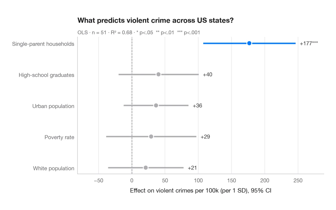
Coefficient plot
Regression estimates with 95% confidence intervals, one row per term.
ggstats::ggcoef_model()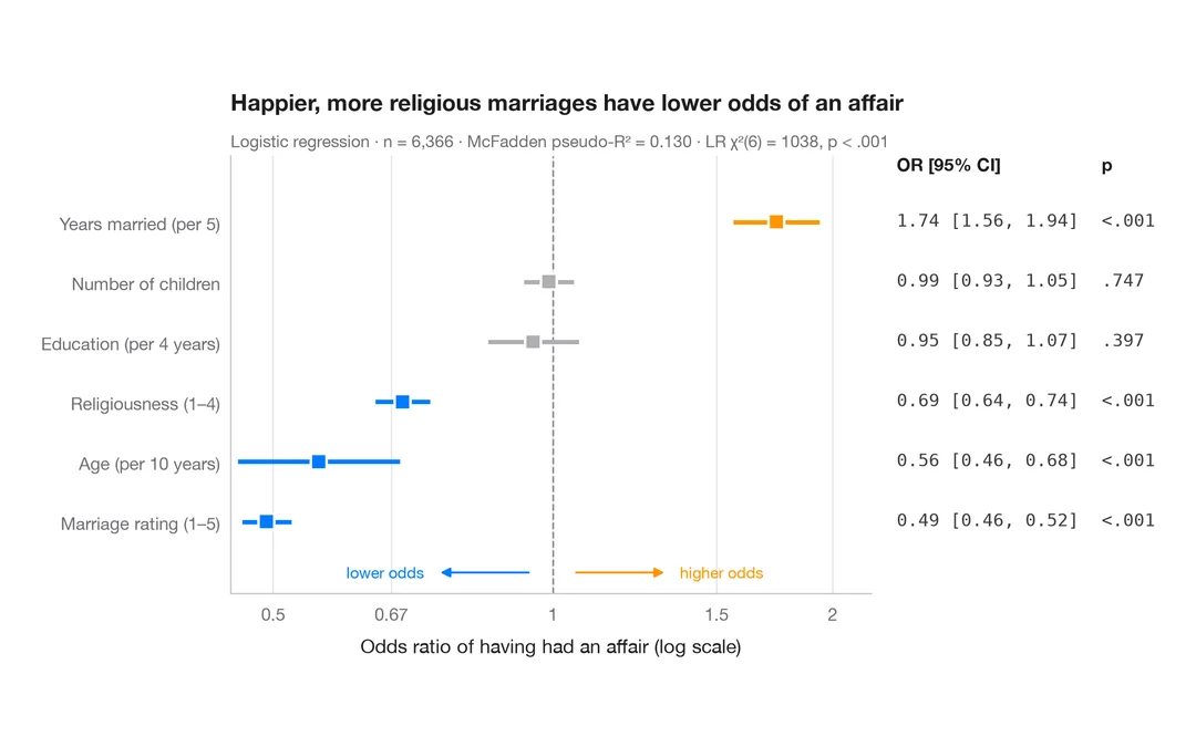
Odds-ratio forest plot
Logistic regression odds ratios on a log scale, with a table of OR [95% CI] alongside.
ggstats::ggcoef_model(exponentiate = TRUE)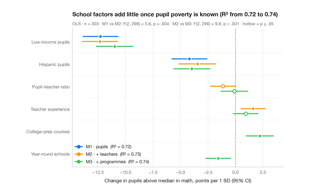
Comparing nested models
Coefficients of three nested regressions of district math results side by side, to see how estimates shift as blocks are added.
ggstats::ggcoef_compare()