Odds-ratio forest plot

Warin, Thierry

Logistic regression odds ratios on a log scale, with a table of OR [95% CI] alongside.

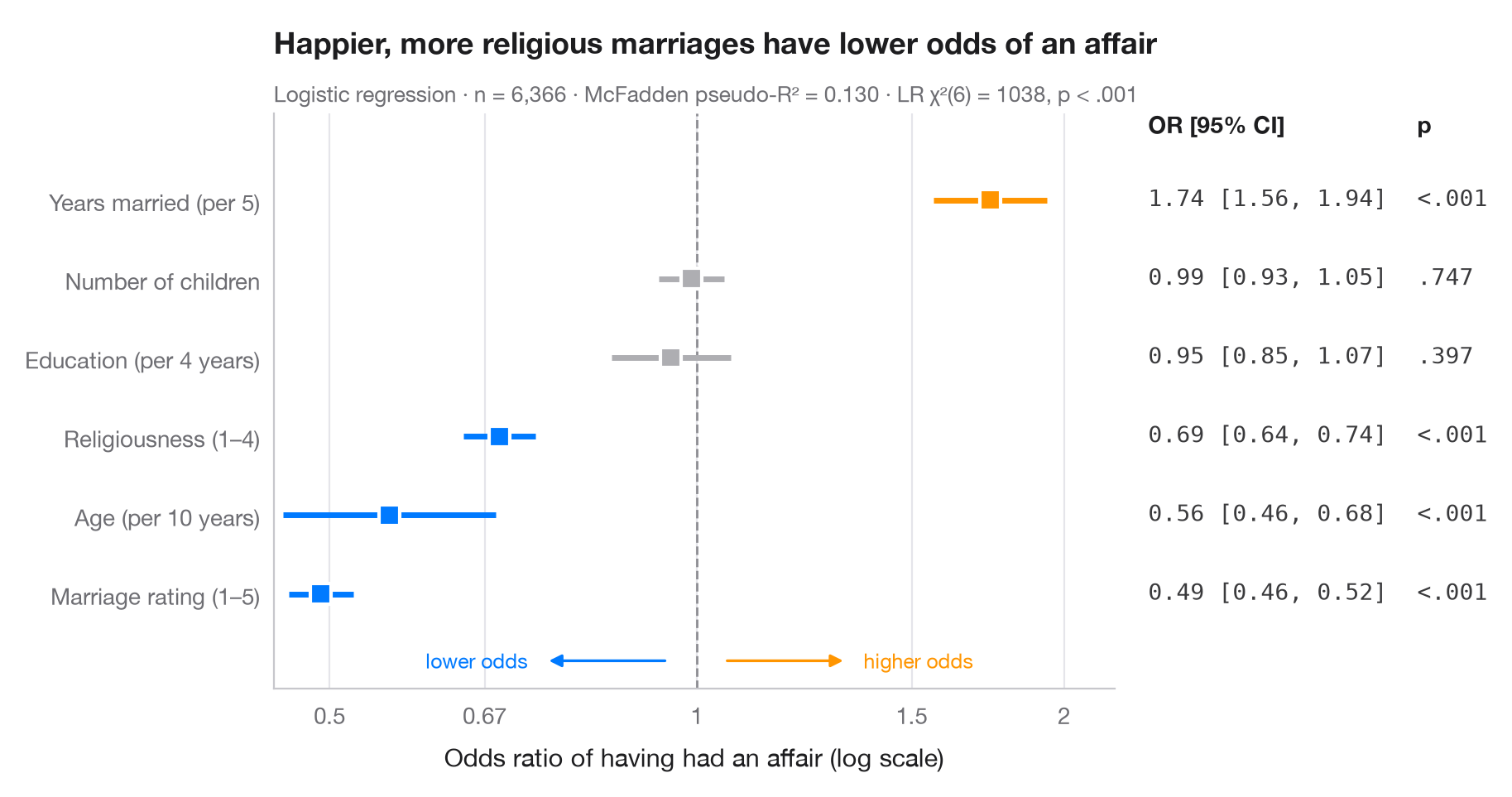
Logistic coefficients are log-odds; exponentiated, they become odds ratios. Each point is the multiplicative change in the odds of the outcome for a one-unit change in the predictor, the line is its 95% confidence interval, and the dashed line at OR = 1 means "no effect". Because ratios are symmetric on a log scale (0.5 is as strong as 2), the x-axis is logarithmic. The right-hand column repeats the numbers, just like the table in a paper.

Data are the 1974 Redbook survey of 6,366 married women bundled with statsmodels (sm.datasets.fair). The outcome is whether the respondent reported any extramarital affair; the model is fitted with smf.logit() and the odds ratios are np.exp() of params and conf_int().

odds-ratio-forest.py · 59 lines

Download GitHub

import matplotlib.pyplot as plt
import numpy as np
import statsmodels.api as sm
import statsmodels.formula.api as smf
from matplotlib.ticker import FixedLocator, NullLocator

# Data: Fair's affairs survey; rescale a few predictors to meaningful units
df = sm.datasets.fair.load_pandas().data
df = df.assign(affair=(df.affairs > 0).astype(int), age10=df.age / 10,
               yrs5=df.yrs_married / 5, educ4=df.educ / 4)

model = smf.logit("affair ~ rate_marriage + religious + age10 + yrs5 + children + educ4",
                  data=df).fit(disp=False)

# Odds ratios with 95% CI (intercept dropped), sorted by effect
tab = np.exp(model.conf_int().drop("Intercept")).rename(columns={0: "low", 1: "high"})
tab = tab.assign(OR=np.exp(model.params), p=model.pvalues).sort_values("OR")
labels = {"rate_marriage": "Marriage rating (1–5)", "religious": "Religiousness (1–4)",
          "age10": "Age (per 10 years)", "yrs5": "Years married (per 5)",
          "children": "Number of children", "educ4": "Education (per 4 years)"}

fig, ax = plt.subplots(figsize=(8.6, 4.6))
y = np.arange(len(tab))
colors = np.where(tab["p"] < 0.05, np.where(tab["OR"] > 1, "#FF9500", "#007AFF"), "#AEAEB2")

ax.axvline(1, color="#8E8E93", lw=1, ls="--", zorder=1)
ax.hlines(y, tab["low"], tab["high"], color=colors, lw=2.5, zorder=2)
ax.scatter(tab["OR"], y, s=80, marker="s", color=colors, edgecolor="white", lw=1.5, zorder=3)

# Right-hand "table" column: OR [95% CI] and p-value
tr = ax.get_yaxis_transform()
top = len(tab) - 0.15
ax.text(1.04, top, "OR [95% CI]", transform=tr, fontsize=10, fontweight="semibold")
ax.text(1.36, top, "p", transform=tr, fontsize=10, fontweight="semibold")
for yi, (_, r) in zip(y, tab.iterrows()):
    ax.text(1.04, yi, f"{r.OR:.2f} [{r.low:.2f}, {r.high:.2f}]", transform=tr,
            va="center", fontsize=10, color="#3A3A3C", family="monospace")
    ax.text(1.36, yi, "<.001" if r.p < .001 else f"{r.p:.3f}".lstrip("0"), transform=tr,
            va="center", fontsize=10, color="#3A3A3C", family="monospace")

ax.set_xscale("log")
ax.xaxis.set_major_locator(FixedLocator([0.5, 0.67, 1, 1.5, 2]))
ax.xaxis.set_minor_locator(NullLocator())
ax.set_xticklabels(["0.5", "0.67", "1", "1.5", "2"])
ax.set_xlim(0.45, 2.2)
ax.set_yticks(y, [labels[t] for t in tab.index])
ax.set_ylim(-1.2, len(tab) + 0.1)
ax.grid(axis="x"); ax.grid(axis="y", visible=False)
ax.set_xlabel("Odds ratio of having had an affair (log scale)")
# Direction hints along the bottom of the panel
for x0, x1, txt, c in [(0.95, 0.75, "lower odds", "#007AFF"), (1.05, 1.33, "higher odds", "#FF9500")]:
    ax.annotate("", (x1, -0.85), (x0, -0.85), arrowprops=dict(arrowstyle="-|>", color=c, lw=1.2))
    ax.text(x1 * (0.97 if x1 < 1 else 1.03), -0.85, txt, color=c, fontsize=9, va="center",
            ha="right" if x1 < 1 else "left")
ax.set_title("Happier, more religious marriages have lower odds of an affair", pad=26)
ax.text(0, 1.02, f"Logistic regression · n = {int(model.nobs):,} · "
        f"McFadden pseudo-R² = {model.prsquared:.3f} · LR χ²({model.df_model:.0f}) = "
        f"{model.llr:.0f}, p < .001", transform=ax.transAxes, fontsize=9.5, color="#6E6E73")
plt.show()

Figures use the optional PyStatlas style: add plt.style.use("pystatlas.mplstyle") to match the look exactly.

Data source

Redbook survey of married women, 1974 (Fair's affairs data). Fair, R. C. (1978). A theory of extramarital affairs. Journal of Political Economy, 86(1), 45–61. https://doi.org/10.1086/260646
Data from the 1974 Redbook magazine survey; distributed with statsmodels (sm.datasets.fair) with the author's permission.

The examples illustrate statistical methods. Their titles describe what each figure shows in these particular data — often a small, dated or partial sample — not the author's position on the substantive question. For interpretation, context and data quality, rely on the original sources cited here.

How to cite

PyStatlas is created and maintained by Thierry Warin. If it helped your work, please cite it.

Warin, T. (2026). Odds-ratio forest plot. In PyStatlas: A Python Gallery of Statistical Graphics for the Social Sciences. https://warint.github.io/pystatlas/regression-models/odds-ratio-forest/

@misc{warin2026statlas,
  author       = {Warin, Thierry},
  title        = {PyStatlas: A Python Gallery of Statistical Graphics for the Social Sciences},
  year         = {2026},
  howpublished = {\url{https://warint.github.io/pystatlas/}},
  note         = {Source code: https://github.com/warint/pystatlas}
}

More in Regression models

Regression models

Coefficient plot

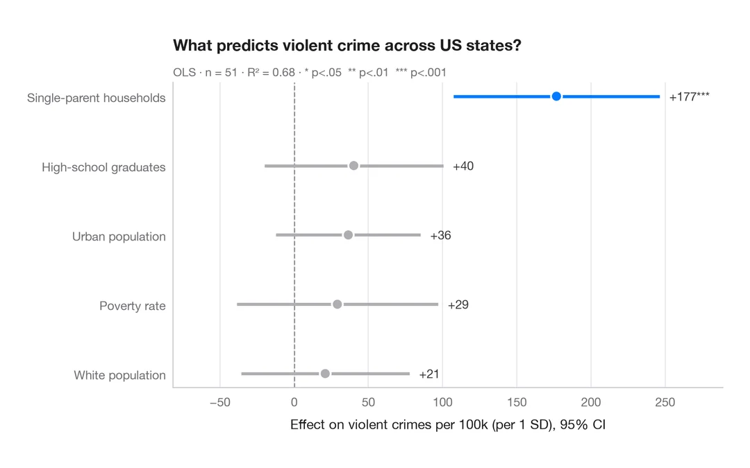
Regression estimates with 95% confidence intervals, one row per term.

ggstats::ggcoef_model()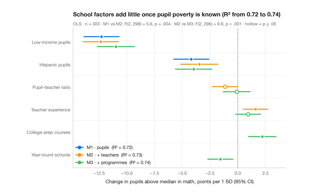

Regression models

Comparing nested models

Coefficients of three nested regressions of district math results side by side, to see how estimates shift as blocks are added.

ggstats::ggcoef_compare()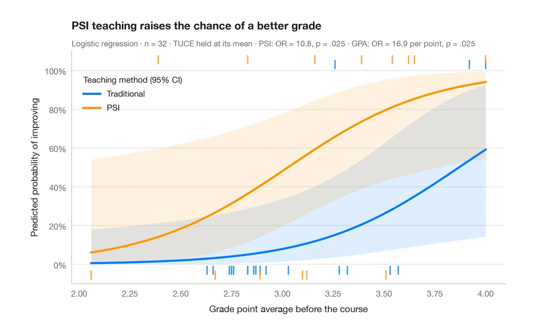

Regression models

Predicted probabilities

Model-based probability curves with 95% CI ribbons across a predictor, by group.

ggeffects::ggpredict() / marginaleffects::plot_predictions()