オッズ比のフォレストプロット
ロジスティック回帰のオッズ比を対数スケールで描き、OR [95% CI] の表を並べます。
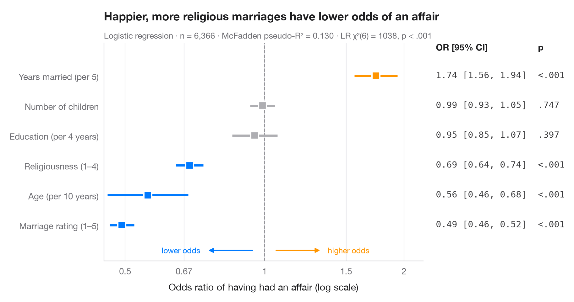
ロジスティック回帰の係数は対数オッズであり、指数変換すると オッズ比 になります。各点は説明変数が1単位変化したときのアウトカムのオッズの乗法的変化、線はその 95% 信頼区間で、OR = 1 の破線は「効果なし」を意味します。比は対数スケール上で対称になる(0.5 は 2 と同じ強さ)ため、x軸は対数軸にしています。右側の列には、論文中の表と同じように数値を再掲しています。
データは statsmodels に同梱されている 1974年の Redbook 誌による既婚女性 6,366 人の調査(sm.datasets.fair)です。アウトカムは回答者が婚外関係を報告したかどうかで、モデルは smf.logit() で当てはめ、オッズ比は params と conf_int() の np.exp() です。
コードおよび図中のテキストは英語です。
import matplotlib.pyplot as plt
import numpy as np
import statsmodels.api as sm
import statsmodels.formula.api as smf
from matplotlib.ticker import FixedLocator, NullLocator

# Data: Fair's affairs survey; rescale a few predictors to meaningful units
df = sm.datasets.fair.load_pandas().data
df = df.assign(affair=(df.affairs > 0).astype(int), age10=df.age / 10,
               yrs5=df.yrs_married / 5, educ4=df.educ / 4)

model = smf.logit("affair ~ rate_marriage + religious + age10 + yrs5 + children + educ4",
                  data=df).fit(disp=False)

# Odds ratios with 95% CI (intercept dropped), sorted by effect
tab = np.exp(model.conf_int().drop("Intercept")).rename(columns={0: "low", 1: "high"})
tab = tab.assign(OR=np.exp(model.params), p=model.pvalues).sort_values("OR")
labels = {"rate_marriage": "Marriage rating (1–5)", "religious": "Religiousness (1–4)",
          "age10": "Age (per 10 years)", "yrs5": "Years married (per 5)",
          "children": "Number of children", "educ4": "Education (per 4 years)"}

fig, ax = plt.subplots(figsize=(8.6, 4.6))
y = np.arange(len(tab))
colors = np.where(tab["p"] < 0.05, np.where(tab["OR"] > 1, "#FF9500", "#007AFF"), "#AEAEB2")

ax.axvline(1, color="#8E8E93", lw=1, ls="--", zorder=1)
ax.hlines(y, tab["low"], tab["high"], color=colors, lw=2.5, zorder=2)
ax.scatter(tab["OR"], y, s=80, marker="s", color=colors, edgecolor="white", lw=1.5, zorder=3)

# Right-hand "table" column: OR [95% CI] and p-value
tr = ax.get_yaxis_transform()
top = len(tab) - 0.15
ax.text(1.04, top, "OR [95% CI]", transform=tr, fontsize=10, fontweight="semibold")
ax.text(1.36, top, "p", transform=tr, fontsize=10, fontweight="semibold")
for yi, (_, r) in zip(y, tab.iterrows()):
    ax.text(1.04, yi, f"{r.OR:.2f} [{r.low:.2f}, {r.high:.2f}]", transform=tr,
            va="center", fontsize=10, color="#3A3A3C", family="monospace")
    ax.text(1.36, yi, "<.001" if r.p < .001 else f"{r.p:.3f}".lstrip("0"), transform=tr,
            va="center", fontsize=10, color="#3A3A3C", family="monospace")

ax.set_xscale("log")
ax.xaxis.set_major_locator(FixedLocator([0.5, 0.67, 1, 1.5, 2]))
ax.xaxis.set_minor_locator(NullLocator())
ax.set_xticklabels(["0.5", "0.67", "1", "1.5", "2"])
ax.set_xlim(0.45, 2.2)
ax.set_yticks(y, [labels[t] for t in tab.index])
ax.set_ylim(-1.2, len(tab) + 0.1)
ax.grid(axis="x"); ax.grid(axis="y", visible=False)
ax.set_xlabel("Odds ratio of having had an affair (log scale)")
# Direction hints along the bottom of the panel
for x0, x1, txt, c in [(0.95, 0.75, "lower odds", "#007AFF"), (1.05, 1.33, "higher odds", "#FF9500")]:
    ax.annotate("", (x1, -0.85), (x0, -0.85), arrowprops=dict(arrowstyle="-|>", color=c, lw=1.2))
    ax.text(x1 * (0.97 if x1 < 1 else 1.03), -0.85, txt, color=c, fontsize=9, va="center",
            ha="right" if x1 < 1 else "left")
ax.set_title("Happier, more religious marriages have lower odds of an affair", pad=26)
ax.text(0, 1.02, f"Logistic regression · n = {int(model.nobs):,} · "
        f"McFadden pseudo-R² = {model.prsquared:.3f} · LR χ²({model.df_model:.0f}) = "
        f"{model.llr:.0f}, p < .001", transform=ax.transAxes, fontsize=9.5, color="#6E6E73")
plt.show()
図にはオプションの PyStatlas スタイル を使用しています。同じ見た目にするには plt.style.use("pystatlas.mplstyle") を追加してください。
データの出典
- Redbook survey of married women, 1974 (Fair's affairs data). Fair, R. C. (1978). A theory of extramarital affairs. Journal of Political Economy, 86(1), 45–61. https://doi.org/10.1086/260646
Data from the 1974 Redbook magazine survey; distributed with statsmodels (sm.datasets.fair) with the author's permission.
これらの例は統計手法を説明するためのものです。図のタイトルは、この特定のデータ(多くは小規模で、古く、部分的な標本)で図が示す内容を述べたものであり、実質的な問いに対する著者の立場ではありません。解釈、背景、データの質については、ここに挙げた元の出典を参照してください。
引用方法
PyStatlas は Thierry Warin が作成・運営しています。研究や業務に役立った場合は、ぜひ引用してください。
Warin, T. (2026). Odds-ratio forest plot. In PyStatlas: A Python Gallery of Statistical Graphics for the Social Sciences. https://warint.github.io/pystatlas/regression-models/odds-ratio-forest/
@misc{warin2026statlas,
  author       = {Warin, Thierry},
  title        = {PyStatlas: A Python Gallery of Statistical Graphics for the Social Sciences},
  year         = {2026},
  howpublished = {\url{https://warint.github.io/pystatlas/}},
  note         = {Source code: https://github.com/warint/pystatlas}
}