入れ子モデルの比較
学区の数学の成績に関する 3 つの入れ子回帰の係数を並べ、ブロックを追加するにつれて推定値がどう動くかを見ます。
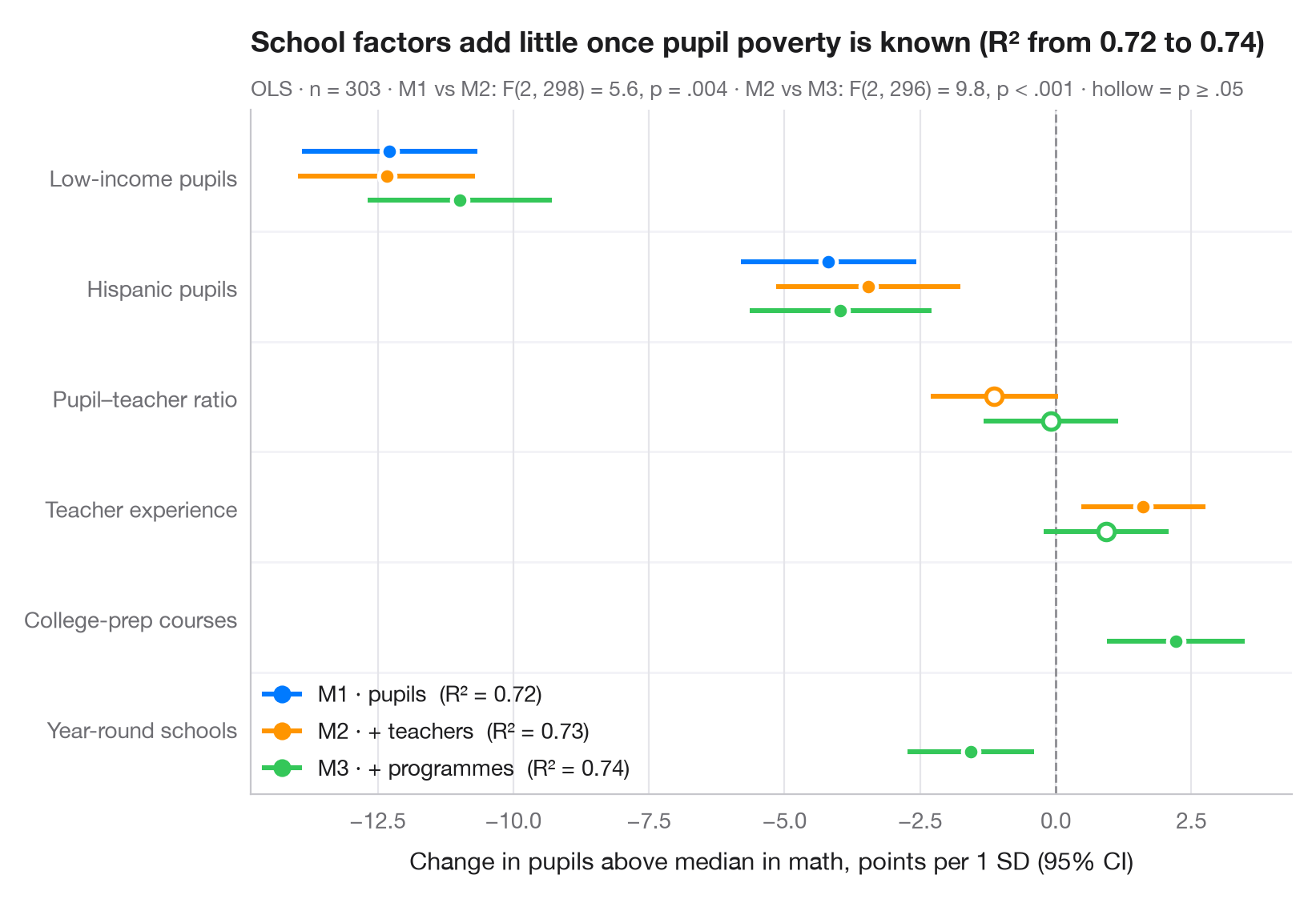
共変量をブロックごとに追加していく場合、注目すべきは どの 項が有意かよりも、推定値がどう動くか であることが少なくありません。ここでは項ごとに1行、モデルごとに少しずらしたドット・アンド・ウィスカーを1つ割り当てているので、モデルが大きくなるにつれて係数がどう変わるかを追えます。白抜きのマーカーは 5% 水準で有意でないことを示します。サブタイトルでは、R² と追加ブロックの F 検定によってモデルを比較しています。
データは statsmodels に同梱されている STAR98 テストのカリフォルニア州 303 学区(sm.datasets.star98)です。目的変数は数学で全国中央値を上回る児童の割合 NABOVE / (NABOVE + NBELOW)(パーセント)です。M1 は児童の構成(低所得とヒスパニック系の児童)、M2 は教員(児童・教員比、平均経験年数)、M3 はプログラム(大学進学準備コース、通年制の学校)を追加します。説明変数は標準化しているので、各係数は 1 標準偏差あたりの変化(パーセントポイント)です。各ブロックは全体として有意ですが、R² はほとんど変わらず、低所得の係数はどのモデルでも −12 前後にとどまります。モデルは smf.ols() で当てはめ、anova_lm() で比較しています。
コードおよび図中のテキストは英語です。
import matplotlib.pyplot as plt
import numpy as np
import statsmodels.api as sm
import statsmodels.formula.api as smf
from statsmodels.stats.anova import anova_lm

# Data: math results in 303 California school districts; standardise predictors (z-scores)
df = sm.datasets.star98.load_pandas().data
df["math"] = 100 * df.NABOVE / (df.NABOVE + df.NBELOW)
X = ["LOWINC", "PERHISP", "PTRATIO", "AVYRSEXP", "PCTAF", "PCTYRRND"]
df[X] = (df[X] - df[X].mean()) / df[X].std()

# Three nested models, each adding a block of predictors
formulas = {"M1 · pupils": "math ~ LOWINC + PERHISP",
            "M2 · + teachers": "math ~ LOWINC + PERHISP + PTRATIO + AVYRSEXP",
            "M3 · + programmes": "math ~ LOWINC + PERHISP + PTRATIO + AVYRSEXP + PCTAF + PCTYRRND"}
fits = {name: smf.ols(f, data=df).fit() for name, f in formulas.items()}
f_tests = anova_lm(*fits.values())

labels = {"LOWINC": "Low-income pupils", "PERHISP": "Hispanic pupils",
          "PTRATIO": "Pupil–teacher ratio", "AVYRSEXP": "Teacher experience",
          "PCTAF": "College-prep courses", "PCTYRRND": "Year-round schools"}
terms = list(labels)[::-1]
palette = ["#007AFF", "#FF9500", "#34C759"]

fig, ax = plt.subplots(figsize=(8, 5.4))
ax.axvline(0, color="#8E8E93", lw=1, ls="--", zorder=1)
for k, ((name, m), c) in enumerate(zip(fits.items(), palette)):
    offset = (1 - k) * 0.22                      # dodge: first model on top
    ci = m.conf_int()
    for i, t in enumerate(terms):
        if t not in m.params:
            continue
        sig = m.pvalues[t] < 0.05
        ax.hlines(i + offset, ci.loc[t, 0], ci.loc[t, 1], color=c, lw=2.2, zorder=2)
        ax.scatter(m.params[t], i + offset, s=55, zorder=3, lw=1.8,
                   color=c if sig else "white", edgecolor=c if not sig else "white")
    ax.plot([], [], "o-", color=c, lw=2.2, ms=7,
            label=f"{name}  (R² = {m.rsquared:.2f})")

for i in range(len(terms) - 1):                  # thin separators between terms
    ax.axhline(i + 0.5, color="#F2F2F7", lw=1, zorder=0)
ax.set_yticks(range(len(terms)), [labels[t] for t in terms])
ax.set_ylim(-0.6, len(terms) - 0.4)
ax.grid(axis="x"); ax.grid(axis="y", visible=False)
ax.set_xlabel("Change in pupils above median in math, points per 1 SD (95% CI)")
ax.legend(loc="lower left", handlelength=1.6, borderaxespad=0.2)
r2 = [m.rsquared for m in fits.values()]
ax.set_title(f"School factors add little once pupil poverty is known (R² from {r2[0]:.2f} to {r2[-1]:.2f})", pad=26)
fmt_p = lambda p: "p < .001" if p < .001 else f"p = {p:.3f}".replace("0.", ".")
blocks = [f"M{j} vs M{j + 1}: F({f_tests.df_diff[j]:.0f}, {f_tests.df_resid[j]:.0f}) = "
          f"{f_tests.F[j]:.1f}, {fmt_p(f_tests['Pr(>F)'][j])}" for j in (1, 2)]
ax.text(0, 1.02, f"OLS · n = {int(fits['M1 · pupils'].nobs)} · " + " · ".join(blocks)
        + " · hollow = p ≥ .05", transform=ax.transAxes, fontsize=9.5, color="#6E6E73")
plt.show()
図にはオプションの PyStatlas スタイル を使用しています。同じ見た目にするには plt.style.use("pystatlas.mplstyle") を追加してください。
データの出典
- California STAR test results, 1998 (303 school districts). Gill, J. (2001). Generalized Linear Models: A Unified Approach (Quantitative Applications in the Social Sciences, No. 134). Sage. https://www.statsmodels.org/stable/datasets/generated/star98.html
Original data from the California Department of Education's Standardized Testing and Reporting (STAR) program, 1998. Subset distributed with statsmodels (sm.datasets.star98) with the author's permission.
これらの例は統計手法を説明するためのものです。図のタイトルは、この特定のデータ(多くは小規模で、古く、部分的な標本)で図が示す内容を述べたものであり、実質的な問いに対する著者の立場ではありません。解釈、背景、データの質については、ここに挙げた元の出典を参照してください。
引用方法
PyStatlas は Thierry Warin が作成・運営しています。研究や業務に役立った場合は、ぜひ引用してください。
Warin, T. (2026). Comparing nested models. In PyStatlas: A Python Gallery of Statistical Graphics for the Social Sciences. https://warint.github.io/pystatlas/regression-models/compare-models/
@misc{warin2026statlas,
  author       = {Warin, Thierry},
  title        = {PyStatlas: A Python Gallery of Statistical Graphics for the Social Sciences},
  year         = {2026},
  howpublished = {\url{https://warint.github.io/pystatlas/}},
  note         = {Source code: https://github.com/warint/pystatlas}
}