Comparing nested models
Coefficients of three nested regressions of district math results side by side, to see how estimates shift as blocks are added.
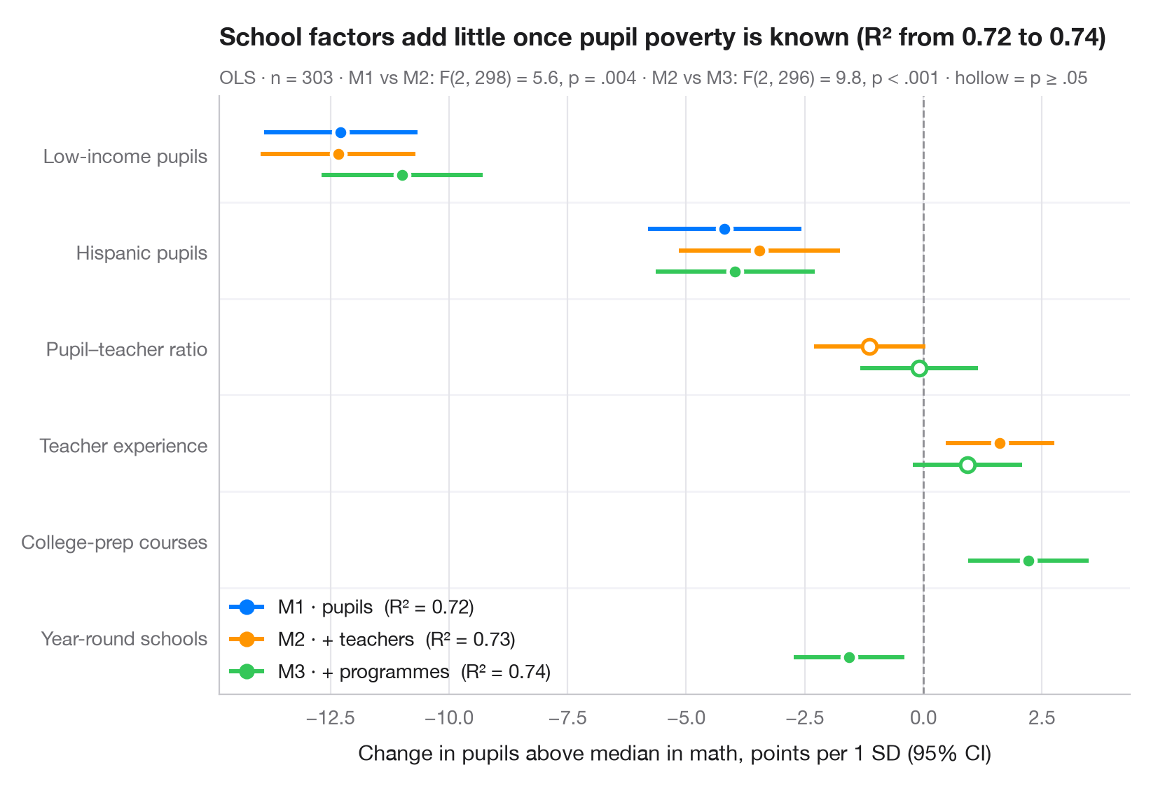
When covariates are added one block at a time, the interesting question is often not which terms are significant but how the estimates move. Here each term gets one row and each model one dodged dot-and-whisker, so you can follow a coefficient as the model grows. Hollow markers are not significant at 5%. The subtitle compares the models with R² and F-tests of the added blocks.
Data are the 303 California school districts of the STAR98 test bundled with
statsmodels (sm.datasets.star98). The outcome is the share of pupils above
the national median in math, NABOVE / (NABOVE + NBELOW), in percent. M1 holds
pupil composition (low-income and Hispanic pupils), M2 adds teachers
(pupil–teacher ratio, average experience) and M3 adds programmes (college-prep
courses, year-round schools). Predictors are standardised, so every coefficient
is the change in percentage points per standard deviation. The blocks are
jointly significant, yet R² barely moves and the low-income coefficient stays
near −12 in every model. Models are fitted with smf.ols() and compared with
anova_lm().
import matplotlib.pyplot as plt
import numpy as np
import statsmodels.api as sm
import statsmodels.formula.api as smf
from statsmodels.stats.anova import anova_lm

# Data: math results in 303 California school districts; standardise predictors (z-scores)
df = sm.datasets.star98.load_pandas().data
df["math"] = 100 * df.NABOVE / (df.NABOVE + df.NBELOW)
X = ["LOWINC", "PERHISP", "PTRATIO", "AVYRSEXP", "PCTAF", "PCTYRRND"]
df[X] = (df[X] - df[X].mean()) / df[X].std()

# Three nested models, each adding a block of predictors
formulas = {"M1 · pupils": "math ~ LOWINC + PERHISP",
            "M2 · + teachers": "math ~ LOWINC + PERHISP + PTRATIO + AVYRSEXP",
            "M3 · + programmes": "math ~ LOWINC + PERHISP + PTRATIO + AVYRSEXP + PCTAF + PCTYRRND"}
fits = {name: smf.ols(f, data=df).fit() for name, f in formulas.items()}
f_tests = anova_lm(*fits.values())

labels = {"LOWINC": "Low-income pupils", "PERHISP": "Hispanic pupils",
          "PTRATIO": "Pupil–teacher ratio", "AVYRSEXP": "Teacher experience",
          "PCTAF": "College-prep courses", "PCTYRRND": "Year-round schools"}
terms = list(labels)[::-1]
palette = ["#007AFF", "#FF9500", "#34C759"]

fig, ax = plt.subplots(figsize=(8, 5.4))
ax.axvline(0, color="#8E8E93", lw=1, ls="--", zorder=1)
for k, ((name, m), c) in enumerate(zip(fits.items(), palette)):
    offset = (1 - k) * 0.22                      # dodge: first model on top
    ci = m.conf_int()
    for i, t in enumerate(terms):
        if t not in m.params:
            continue
        sig = m.pvalues[t] < 0.05
        ax.hlines(i + offset, ci.loc[t, 0], ci.loc[t, 1], color=c, lw=2.2, zorder=2)
        ax.scatter(m.params[t], i + offset, s=55, zorder=3, lw=1.8,
                   color=c if sig else "white", edgecolor=c if not sig else "white")
    ax.plot([], [], "o-", color=c, lw=2.2, ms=7,
            label=f"{name}  (R² = {m.rsquared:.2f})")

for i in range(len(terms) - 1):                  # thin separators between terms
    ax.axhline(i + 0.5, color="#F2F2F7", lw=1, zorder=0)
ax.set_yticks(range(len(terms)), [labels[t] for t in terms])
ax.set_ylim(-0.6, len(terms) - 0.4)
ax.grid(axis="x"); ax.grid(axis="y", visible=False)
ax.set_xlabel("Change in pupils above median in math, points per 1 SD (95% CI)")
ax.legend(loc="lower left", handlelength=1.6, borderaxespad=0.2)
r2 = [m.rsquared for m in fits.values()]
ax.set_title(f"School factors add little once pupil poverty is known (R² from {r2[0]:.2f} to {r2[-1]:.2f})", pad=26)
fmt_p = lambda p: "p < .001" if p < .001 else f"p = {p:.3f}".replace("0.", ".")
blocks = [f"M{j} vs M{j + 1}: F({f_tests.df_diff[j]:.0f}, {f_tests.df_resid[j]:.0f}) = "
          f"{f_tests.F[j]:.1f}, {fmt_p(f_tests['Pr(>F)'][j])}" for j in (1, 2)]
ax.text(0, 1.02, f"OLS · n = {int(fits['M1 · pupils'].nobs)} · " + " · ".join(blocks)
        + " · hollow = p ≥ .05", transform=ax.transAxes, fontsize=9.5, color="#6E6E73")
plt.show()
Figures use the optional PyStatlas style: add plt.style.use("pystatlas.mplstyle") to match the look exactly.
Data source
- California STAR test results, 1998 (303 school districts). Gill, J. (2001). Generalized Linear Models: A Unified Approach (Quantitative Applications in the Social Sciences, No. 134). Sage. https://www.statsmodels.org/stable/datasets/generated/star98.html
Original data from the California Department of Education's Standardized Testing and Reporting (STAR) program, 1998. Subset distributed with statsmodels (sm.datasets.star98) with the author's permission.
The examples illustrate statistical methods. Their titles describe what each figure shows in these particular data — often a small, dated or partial sample — not the author's position on the substantive question. For interpretation, context and data quality, rely on the original sources cited here.
How to cite
PyStatlas is created and maintained by Thierry Warin. If it helped your work, please cite it.
Warin, T. (2026). Comparing nested models. In PyStatlas: A Python Gallery of Statistical Graphics for the Social Sciences. https://warint.github.io/pystatlas/regression-models/compare-models/
@misc{warin2026statlas,
  author       = {Warin, Thierry},
  title        = {PyStatlas: A Python Gallery of Statistical Graphics for the Social Sciences},
  year         = {2026},
  howpublished = {\url{https://warint.github.io/pystatlas/}},
  note         = {Source code: https://github.com/warint/pystatlas}
}More in Regression models
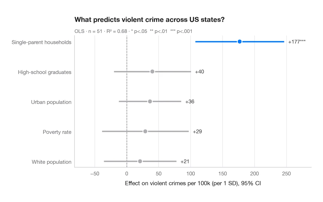
Coefficient plot
Regression estimates with 95% confidence intervals, one row per term.
ggstats::ggcoef_model()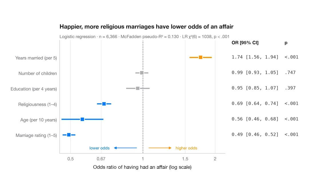
Odds-ratio forest plot
Logistic regression odds ratios on a log scale, with a table of OR [95% CI] alongside.
ggstats::ggcoef_model(exponentiate = TRUE)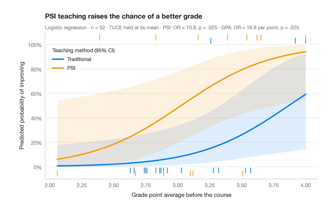
Predicted probabilities
Model-based probability curves with 95% CI ribbons across a predictor, by group.
ggeffects::ggpredict() / marginaleffects::plot_predictions()