Interaction effects
Simple slopes at mean ± 1 SD and a Johnson–Neyman plot for college-prep courses and math results, moderated by pupil poverty.
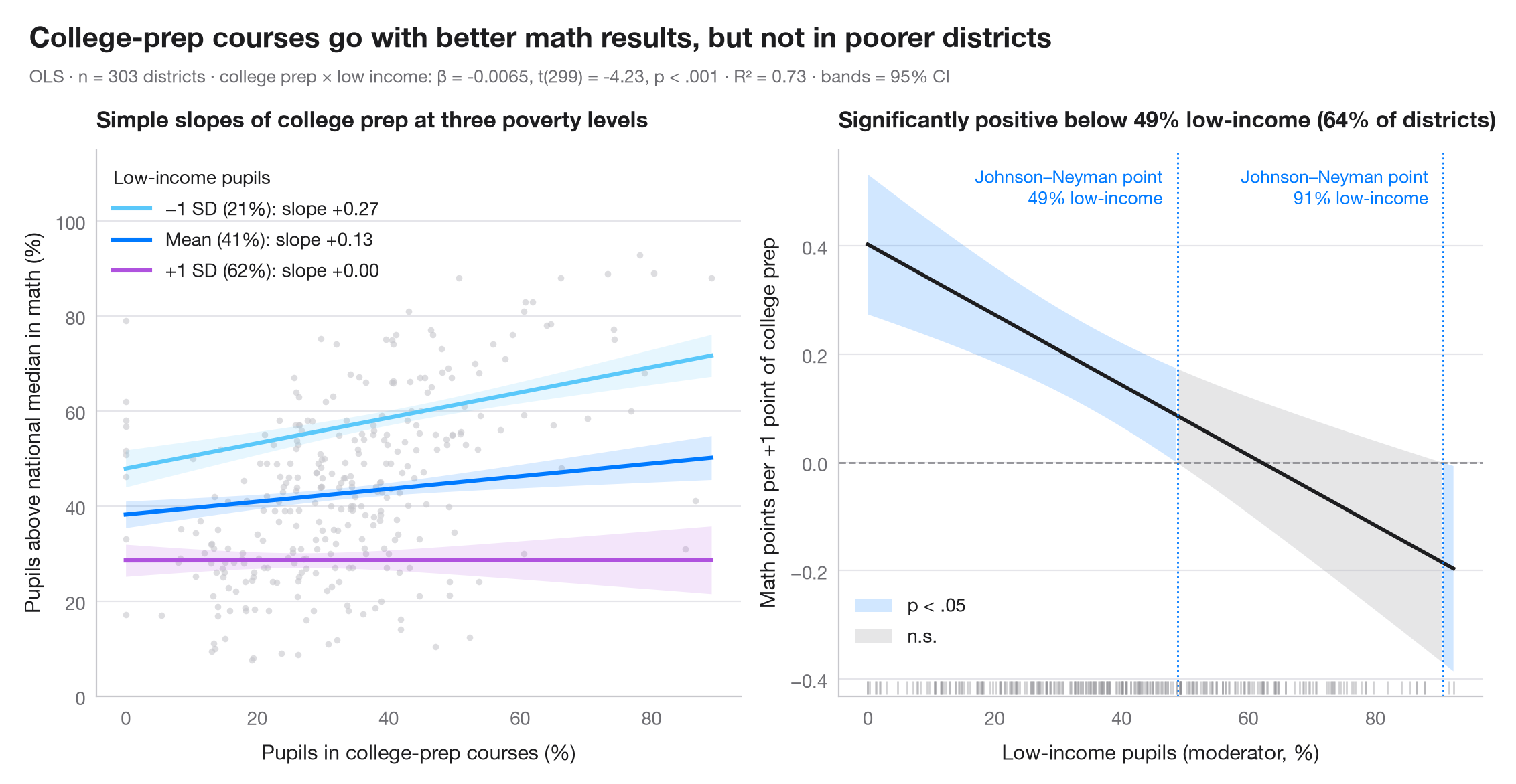
An interaction term says that the slope of one predictor depends on another. The left panel draws that slope at three values of the moderator — its mean and ±1 standard deviation — each with a 95% confidence band. The right panel is the Johnson–Neyman view: the marginal effect of the focal predictor, β₁ + β₃·moderator, across the whole range of the moderator, with its 95% CI. Where the band excludes zero the effect is significant; the switch-over is the Johnson–Neyman point.
Data are the 303 California school districts of the STAR98 test bundled with
statsmodels (sm.datasets.star98). The outcome is the share of pupils above
the national median in math (%); the focal predictor is the share of pupils in
college-prep (UC/CSU) courses and the moderator the share of low-income pupils,
in smf.ols("math ~ prep * lowinc"). College-prep enrolment goes with better
math results in better-off districts, but the association fades as poverty
rises — and turns significantly negative only in the two poorest districts,
hence a second Johnson–Neyman point at the far right. The marginal-effect
variance is computed by hand from cov_params():
Var(β₁) + 2m·Cov(β₁, β₃) + m²·Var(β₃).
import matplotlib.pyplot as plt
import numpy as np
import pandas as pd
import statsmodels.api as sm
import statsmodels.formula.api as smf
from scipy import stats

# Data: math results, college-prep enrolment and low-income pupils in 303 California districts
raw = sm.datasets.star98.load_pandas().data
df = pd.DataFrame({"math": 100 * raw.NABOVE / (raw.NABOVE + raw.NBELOW),
                   "prep": raw.PCTAF, "lowinc": raw.LOWINC})
model = smf.ols("math ~ prep * lowinc", data=df).fit()
b, V = model.params, model.cov_params()
t_crit = stats.t.ppf(0.975, model.df_resid)

fig, (ax1, ax2) = plt.subplots(1, 2, figsize=(11, 5))

# Left: simple slopes of college prep at low income = mean − 1 SD, mean, mean + 1 SD
ax1.scatter(df.prep, df.math, s=12, color="#C7C7CC", alpha=0.6, lw=0)
prep = np.linspace(df.prep.min(), df.prep.max(), 100)
m, s = df.lowinc.mean(), df.lowinc.std()
for low, lab, c in [(m - s, "−1 SD", "#5AC8FA"), (m, "Mean", "#007AFF"), (m + s, "+1 SD", "#AF52DE")]:
    pred = model.get_prediction(pd.DataFrame({"prep": prep, "lowinc": low})).summary_frame()
    ax1.fill_between(prep, pred.mean_ci_lower, pred.mean_ci_upper, color=c, alpha=0.15, lw=0)
    ax1.plot(prep, pred["mean"], color=c, lw=2.2,
             label=f"{lab} ({low:.0f}%): slope {b['prep'] + b['prep:lowinc'] * low:+.2f}")
ax1.legend(title="Low-income pupils", loc="upper left", alignment="left")
ax1.set_ylim(0, 115)
ax1.set_xlabel("Pupils in college-prep courses (%)")
ax1.set_ylabel("Pupils above national median in math (%)")
ax1.set_title("Simple slopes of college prep at three poverty levels", fontsize=12)

# Right: Johnson–Neyman — marginal effect of college prep across low income, with 95% CI
lowinc = np.linspace(df.lowinc.min(), df.lowinc.max(), 400)
eff = b["prep"] + b["prep:lowinc"] * lowinc
se = np.sqrt(V.loc["prep", "prep"] + 2 * lowinc * V.loc["prep", "prep:lowinc"]
             + lowinc**2 * V.loc["prep:lowinc", "prep:lowinc"])
lo, hi = eff - t_crit * se, eff + t_crit * se
sig = (lo > 0) | (hi < 0)
ax2.axhline(0, color="#8E8E93", lw=1, ls="--")
ax2.fill_between(lowinc, lo, hi, where=sig, color="#007AFF", alpha=0.18, lw=0, label="p < .05")
ax2.fill_between(lowinc, lo, hi, where=~sig, color="#AEAEB2", alpha=0.3, lw=0, label="n.s.")
ax2.plot(lowinc, eff, color="#1D1D1F", lw=2)
jns = lowinc[1:][np.diff(sig.astype(int)) != 0]     # where significance switches
for jn in jns:
    ax2.axvline(jn, color="#007AFF", lw=1, ls=":")
    ax2.annotate(f"Johnson–Neyman point\n{jn:.0f}% low-income", (jn, 0.97), xytext=(-8, 0),
                 xycoords=ax2.get_xaxis_transform(), textcoords="offset points",
                 fontsize=9.5, color="#007AFF", va="top", ha="right")
# Rug of the observed moderator values
ax2.plot(df.lowinc, np.full(len(df), 0.015), "|", ms=7, color="#8E8E93", alpha=0.4,
         transform=ax2.get_xaxis_transform())
share = (df.lowinc < jns[0]).mean()
ax2.legend(loc="lower left", bbox_to_anchor=(0, 0.06))
ax2.set_xlabel("Low-income pupils (moderator, %)")
ax2.set_ylabel("Math points per +1 point of college prep")
ax2.set_title(f"Significantly positive below {jns[0]:.0f}% low-income ({share:.0%} of districts)", fontsize=12)

# Figure title and statistical subtitle above both panels
p_int = model.pvalues["prep:lowinc"]
p_txt = "p < .001" if p_int < 0.001 else f"p = {p_int:.3f}"
fig.text(0.01, 1.07, "College-prep courses go with better math results, but not in poorer districts",
         fontsize=15, fontweight="semibold", va="bottom")
fig.text(0.01, 1.02, f"OLS · n = {int(model.nobs)} districts · college prep × low income: β = {b['prep:lowinc']:.4f}, "
         f"t({model.df_resid:.0f}) = {model.tvalues['prep:lowinc']:.2f}, "
         f"{p_txt} · R² = {model.rsquared:.2f} · bands = 95% CI",
         fontsize=9.5, color="#6E6E73", va="bottom")
plt.show()
Figures use the optional PyStatlas style: add plt.style.use("pystatlas.mplstyle") to match the look exactly.
Data source
- California STAR test results, 1998 (303 school districts). Gill, J. (2001). Generalized Linear Models: A Unified Approach (Quantitative Applications in the Social Sciences, No. 134). Sage. https://www.statsmodels.org/stable/datasets/generated/star98.html
Original data from the California Department of Education's Standardized Testing and Reporting (STAR) program, 1998. Subset distributed with statsmodels (sm.datasets.star98) with the author's permission.
The examples illustrate statistical methods. Their titles describe what each figure shows in these particular data — often a small, dated or partial sample — not the author's position on the substantive question. For interpretation, context and data quality, rely on the original sources cited here.
How to cite
PyStatlas is created and maintained by Thierry Warin. If it helped your work, please cite it.
Warin, T. (2026). Interaction effects. In PyStatlas: A Python Gallery of Statistical Graphics for the Social Sciences. https://warint.github.io/pystatlas/regression-models/interaction-effects/
@misc{warin2026statlas,
  author       = {Warin, Thierry},
  title        = {PyStatlas: A Python Gallery of Statistical Graphics for the Social Sciences},
  year         = {2026},
  howpublished = {\url{https://warint.github.io/pystatlas/}},
  note         = {Source code: https://github.com/warint/pystatlas}
}More in Regression models
Coefficient plot
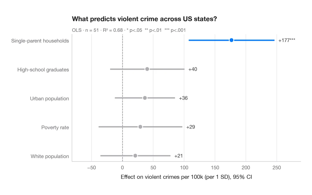
Regression estimates with 95% confidence intervals, one row per term.
ggstats::ggcoef_model()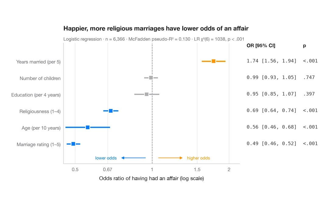
Odds-ratio forest plot
Logistic regression odds ratios on a log scale, with a table of OR [95% CI] alongside.
ggstats::ggcoef_model(exponentiate = TRUE)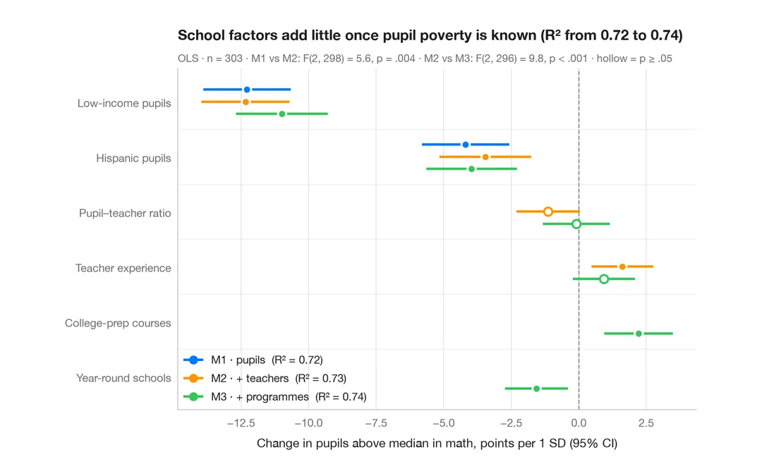
Comparing nested models
Coefficients of three nested regressions of district math results side by side, to see how estimates shift as blocks are added.
ggstats::ggcoef_compare()