Pairs plot with correlations
Scatter matrix of four school-district variables, with group KDEs on the diagonal and pooled vs within-group correlations above it.
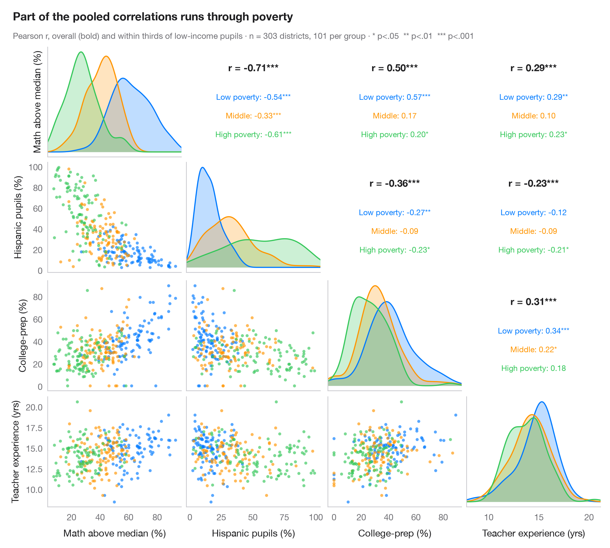
The Python counterpart of GGally::ggpairs(). Every pair of variables gets a
scatterplot below the diagonal, coloured by group; the diagonal shows each
variable's density per group; and the mirror cell above the diagonal prints
Pearson's r, overall (bold) and within each group, with significance stars.
Comparing the two is the point: pooled and within-group correlations can differ
sharply — even in sign — when groups sit in different regions of the plot.
Data are the 303 California school districts of the STAR98 test bundled with
statsmodels (sm.datasets.star98): the share of pupils above the national
median in math, the shares of Hispanic pupils and of pupils in college-prep
(UC/CSU) courses, and teachers' average years of experience. Districts are
grouped into thirds of their share of low-income pupils (pd.qcut, 101 each),
so the within-group coefficients hold poverty roughly constant: the link
between Hispanic share and math results, −0.71 overall, is weaker inside every
poverty group. Densities use scipy.stats.gaussian_kde and correlations
scipy.stats.pearsonr; the grid is a plain plt.subplots(4, 4).
import matplotlib.pyplot as plt
import numpy as np
import pandas as pd
import statsmodels.api as sm
from scipy import stats

# Data: 303 California school districts (STAR98), grouped by thirds of low-income pupils
raw = sm.datasets.star98.load_pandas().data
df = pd.DataFrame({"Math above median (%)": 100 * raw.NABOVE / (raw.NABOVE + raw.NBELOW),
                   "Hispanic pupils (%)": raw.PERHISP, "College-prep (%)": raw.PCTAF,
                   "Teacher experience (yrs)": raw.AVYRSEXP})
groups = ["Low poverty", "Middle", "High poverty"]
df["group"] = pd.qcut(raw.LOWINC, 3, labels=groups).astype(str)
cols = df.columns[:4]
palette = ["#007AFF", "#FF9500", "#34C759"]
stars = lambda p: "***" if p < .001 else "**" if p < .01 else "*" if p < .05 else ""

fig, axes = plt.subplots(4, 4, figsize=(9.5, 8.6), sharex="col")
lims = {c: (df[c].min() - 0.05 * np.ptp(df[c]), df[c].max() + 0.05 * np.ptp(df[c])) for c in cols}
fig.get_layout_engine().set(rect=(0, 0, 1, 0.92), w_pad=0.04, h_pad=0.04)
for i, yv in enumerate(cols):
    for j, xv in enumerate(cols):
        ax = axes[i, j]
        ax.grid(False)
        if i == j:                                       # diagonal: KDE per group
            grid = np.linspace(*lims[xv], 200)
            for s, c in zip(groups, palette):
                dens = stats.gaussian_kde(df.loc[df.group == s, xv])(grid)
                ax.fill_between(grid, dens, color=c, alpha=0.25, lw=0)
                ax.plot(grid, dens, color=c, lw=1.3)
            ax.set_yticks([])
        elif i > j:                                      # lower: scatter by group
            for s, c in zip(groups, palette):
                d = df[df.group == s]
                ax.scatter(d[xv], d[yv], s=12, color=c, alpha=0.65, lw=0)
            ax.set_ylim(lims[yv])
        else:                                            # upper: correlation coefficients
            r, p = stats.pearsonr(df[xv], df[yv])
            ax.text(0.5, 0.78, f"r = {r:.2f}{stars(p)}", ha="center", fontsize=11,
                    fontweight="semibold", transform=ax.transAxes)
            for k, (s, c) in enumerate(zip(groups, palette)):
                d = df[df.group == s]
                rs, ps = stats.pearsonr(d[xv], d[yv])
                ax.text(0.5, 0.52 - k * 0.17, f"{s}: {rs:.2f}{stars(ps)}", ha="center",
                        fontsize=9, color=c, transform=ax.transAxes)
            ax.tick_params(labelbottom=False, labelleft=False)
            for sp in ax.spines.values():
                sp.set_visible(False)
        if i < 3:
            ax.tick_params(labelbottom=False)
        if j > 0 or i == 0:
            ax.tick_params(labelleft=False)
        if i == 3:
            ax.set_xlabel(xv)
            ax.set_xlim(lims[xv])
        if j == 0:
            ax.set_ylabel(yv)

fig.text(0.01, 0.985, "Part of the pooled correlations runs through poverty", fontsize=13,
         fontweight="semibold", va="top")
fig.text(0.01, 0.945, f"Pearson r, overall (bold) and within thirds of low-income pupils · n = {len(df)} "
         "districts, 101 per group · * p<.05  ** p<.01  *** p<.001", fontsize=9.5, color="#6E6E73", va="top")
plt.show()
Figures use the optional PyStatlas style: add plt.style.use("pystatlas.mplstyle") to match the look exactly.
Data source
- California STAR test results, 1998 (303 school districts). Gill, J. (2001). Generalized Linear Models: A Unified Approach (Quantitative Applications in the Social Sciences, No. 134). Sage. https://www.statsmodels.org/stable/datasets/generated/star98.html
Original data from the California Department of Education's Standardized Testing and Reporting (STAR) program, 1998. Subset distributed with statsmodels (sm.datasets.star98) with the author's permission.
The examples illustrate statistical methods. Their titles describe what each figure shows in these particular data — often a small, dated or partial sample — not the author's position on the substantive question. For interpretation, context and data quality, rely on the original sources cited here.
How to cite
PyStatlas is created and maintained by Thierry Warin. If it helped your work, please cite it.
Warin, T. (2026). Pairs plot with correlations. In PyStatlas: A Python Gallery of Statistical Graphics for the Social Sciences. https://warint.github.io/pystatlas/correlation/pairs-plot/
@misc{warin2026statlas,
  author       = {Warin, Thierry},
  title        = {PyStatlas: A Python Gallery of Statistical Graphics for the Social Sciences},
  year         = {2026},
  howpublished = {\url{https://warint.github.io/pystatlas/}},
  note         = {Source code: https://github.com/warint/pystatlas}
}More in Correlation & association
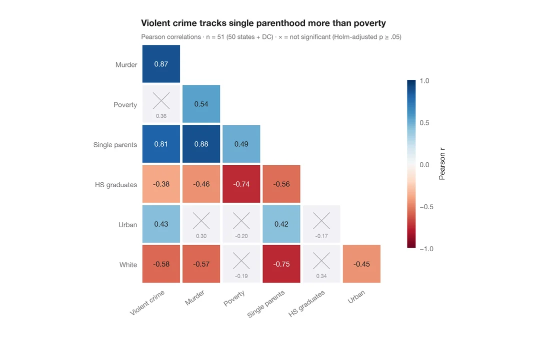
Correlation matrix
Lower-triangle Pearson correlation heatmap; non-significant cells (Holm) are crossed out.
ggstatsplot::ggcorrmat()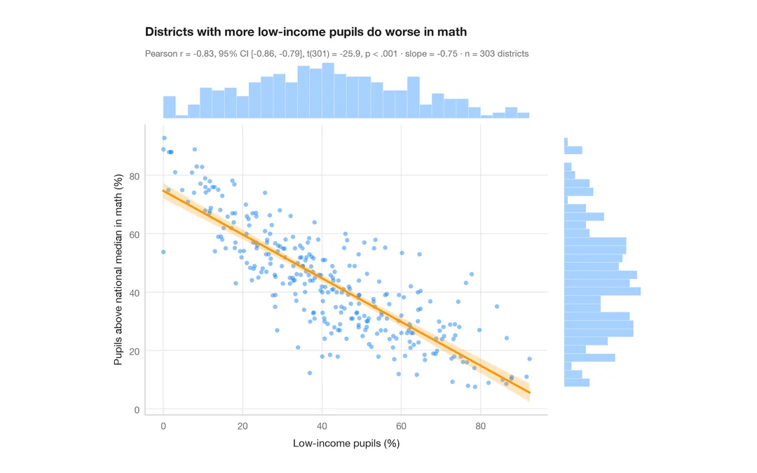
Scatterplot with statistics
Low-income pupils vs math results in 303 California districts — scatter, OLS line with 95% band, marginal histograms and Pearson's r.
ggstatsplot::ggscatterstats()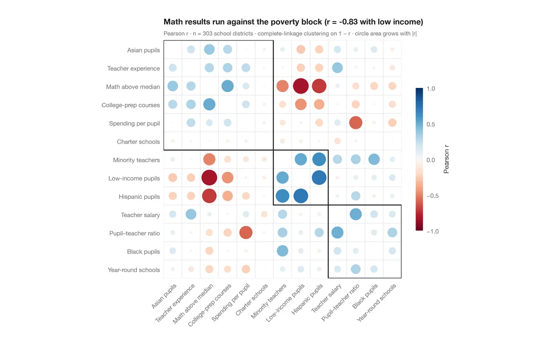
Correlogram with clustering
Corrplot-style circles sized and coloured by r for 13 school-district indicators, ordered by hierarchical clustering.
corrplot::corrplot(order = "hclust", addrect = 3)