相関係数付きペアプロット
学区に関する 4 変数の散布図行列。対角線上に群別の密度、その上に全体と群内の相関係数を示します。
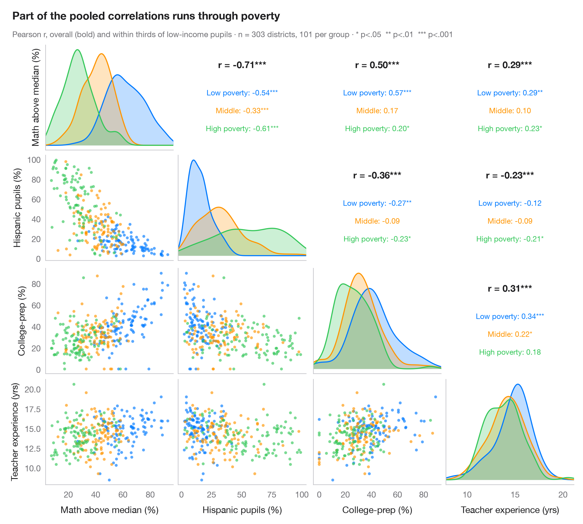
GGally::ggpairs() の Python 版です。対角線より下には変数の各ペアの散布図を群ごとに色分けして描き、対角線上には各変数の群別の密度を示し、対角線より上の対称なセルにはピアソンの r を全体(太字)と群ごとに有意性の星印付きで表示しています。この2つを比べることが要点です。群がプロットの異なる領域に位置していると、全体の相関と群内の相関は大きく異なり、符号が逆になることさえあります。
データは statsmodels に同梱されている STAR98 テストのカリフォルニア州 303 学区(sm.datasets.star98)です。数学で全国中央値を上回る児童の割合、ヒスパニック系児童の割合、大学進学準備(UC/CSU)コースを履修する生徒の割合、教員の平均経験年数を用いています。学区は低所得世帯の児童の割合によって 3 等分され(pd.qcut、各 101 学区)、群内の係数では貧困の水準がほぼ一定に保たれます。ヒスパニック系の割合と数学の成績との関連は全体では −0.71 ですが、どの貧困群の中でもそれより弱くなります。密度は scipy.stats.gaussian_kde、相関は scipy.stats.pearsonr で計算し、グリッドは単純な plt.subplots(4, 4) です。
コードおよび図中のテキストは英語です。
import matplotlib.pyplot as plt
import numpy as np
import pandas as pd
import statsmodels.api as sm
from scipy import stats

# Data: 303 California school districts (STAR98), grouped by thirds of low-income pupils
raw = sm.datasets.star98.load_pandas().data
df = pd.DataFrame({"Math above median (%)": 100 * raw.NABOVE / (raw.NABOVE + raw.NBELOW),
                   "Hispanic pupils (%)": raw.PERHISP, "College-prep (%)": raw.PCTAF,
                   "Teacher experience (yrs)": raw.AVYRSEXP})
groups = ["Low poverty", "Middle", "High poverty"]
df["group"] = pd.qcut(raw.LOWINC, 3, labels=groups).astype(str)
cols = df.columns[:4]
palette = ["#007AFF", "#FF9500", "#34C759"]
stars = lambda p: "***" if p < .001 else "**" if p < .01 else "*" if p < .05 else ""

fig, axes = plt.subplots(4, 4, figsize=(9.5, 8.6), sharex="col")
lims = {c: (df[c].min() - 0.05 * np.ptp(df[c]), df[c].max() + 0.05 * np.ptp(df[c])) for c in cols}
fig.get_layout_engine().set(rect=(0, 0, 1, 0.92), w_pad=0.04, h_pad=0.04)
for i, yv in enumerate(cols):
    for j, xv in enumerate(cols):
        ax = axes[i, j]
        ax.grid(False)
        if i == j:                                       # diagonal: KDE per group
            grid = np.linspace(*lims[xv], 200)
            for s, c in zip(groups, palette):
                dens = stats.gaussian_kde(df.loc[df.group == s, xv])(grid)
                ax.fill_between(grid, dens, color=c, alpha=0.25, lw=0)
                ax.plot(grid, dens, color=c, lw=1.3)
            ax.set_yticks([])
        elif i > j:                                      # lower: scatter by group
            for s, c in zip(groups, palette):
                d = df[df.group == s]
                ax.scatter(d[xv], d[yv], s=12, color=c, alpha=0.65, lw=0)
            ax.set_ylim(lims[yv])
        else:                                            # upper: correlation coefficients
            r, p = stats.pearsonr(df[xv], df[yv])
            ax.text(0.5, 0.78, f"r = {r:.2f}{stars(p)}", ha="center", fontsize=11,
                    fontweight="semibold", transform=ax.transAxes)
            for k, (s, c) in enumerate(zip(groups, palette)):
                d = df[df.group == s]
                rs, ps = stats.pearsonr(d[xv], d[yv])
                ax.text(0.5, 0.52 - k * 0.17, f"{s}: {rs:.2f}{stars(ps)}", ha="center",
                        fontsize=9, color=c, transform=ax.transAxes)
            ax.tick_params(labelbottom=False, labelleft=False)
            for sp in ax.spines.values():
                sp.set_visible(False)
        if i < 3:
            ax.tick_params(labelbottom=False)
        if j > 0 or i == 0:
            ax.tick_params(labelleft=False)
        if i == 3:
            ax.set_xlabel(xv)
            ax.set_xlim(lims[xv])
        if j == 0:
            ax.set_ylabel(yv)

fig.text(0.01, 0.985, "Part of the pooled correlations runs through poverty", fontsize=13,
         fontweight="semibold", va="top")
fig.text(0.01, 0.945, f"Pearson r, overall (bold) and within thirds of low-income pupils · n = {len(df)} "
         "districts, 101 per group · * p<.05  ** p<.01  *** p<.001", fontsize=9.5, color="#6E6E73", va="top")
plt.show()
図にはオプションの PyStatlas スタイル を使用しています。同じ見た目にするには plt.style.use("pystatlas.mplstyle") を追加してください。
データの出典
- California STAR test results, 1998 (303 school districts). Gill, J. (2001). Generalized Linear Models: A Unified Approach (Quantitative Applications in the Social Sciences, No. 134). Sage. https://www.statsmodels.org/stable/datasets/generated/star98.html
Original data from the California Department of Education's Standardized Testing and Reporting (STAR) program, 1998. Subset distributed with statsmodels (sm.datasets.star98) with the author's permission.
これらの例は統計手法を説明するためのものです。図のタイトルは、この特定のデータ(多くは小規模で、古く、部分的な標本)で図が示す内容を述べたものであり、実質的な問いに対する著者の立場ではありません。解釈、背景、データの質については、ここに挙げた元の出典を参照してください。
引用方法
PyStatlas は Thierry Warin が作成・運営しています。研究や業務に役立った場合は、ぜひ引用してください。
Warin, T. (2026). Pairs plot with correlations. In PyStatlas: A Python Gallery of Statistical Graphics for the Social Sciences. https://warint.github.io/pystatlas/correlation/pairs-plot/
@misc{warin2026statlas,
  author       = {Warin, Thierry},
  title        = {PyStatlas: A Python Gallery of Statistical Graphics for the Social Sciences},
  year         = {2026},
  howpublished = {\url{https://warint.github.io/pystatlas/}},
  note         = {Source code: https://github.com/warint/pystatlas}
}相関と関連のその他のグラフ
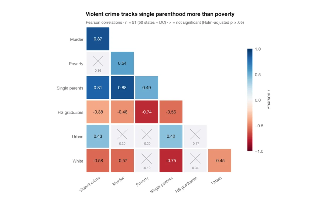
相関行列
ピアソン相関の下三角ヒートマップ。有意でないセル(ホルム法)には×印を付けます。
ggstatsplot::ggcorrmat()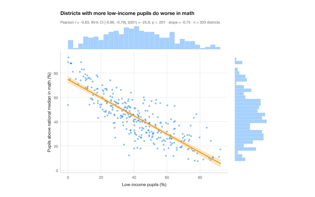
統計量付き散布図
カリフォルニア州 303 学区における低所得世帯の児童の割合と数学の成績 — 散布図、95% 信頼帯付きの OLS 直線、周辺ヒストグラム、ピアソンの r。
ggstatsplot::ggscatterstats()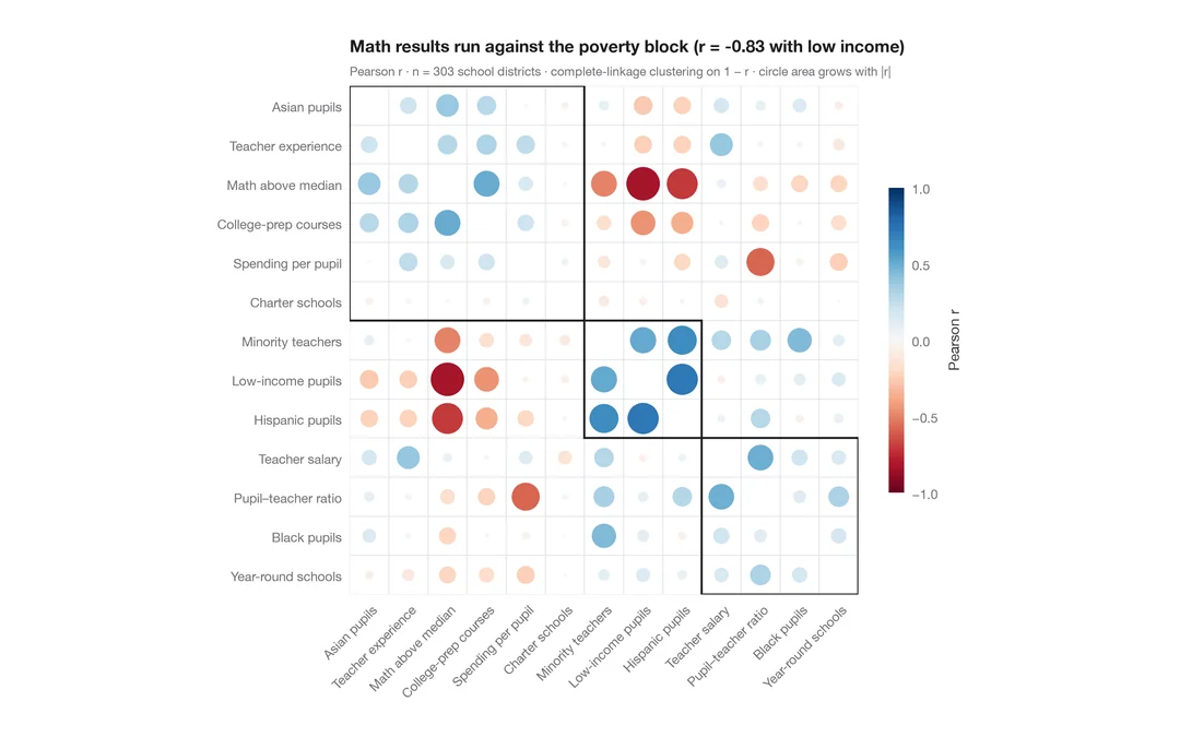
クラスタリング付きコレログラム
学区に関する 13 の指標について、r に応じて大きさと色を決めた corrplot 風の円を、階層的クラスタリングの順に並べたものです。
corrplot::corrplot(order = "hclust", addrect = 3)