統計量付き散布図
カリフォルニア州 303 学区における低所得世帯の児童の割合と数学の成績 — 散布図、95% 信頼帯付きの OLS 直線、周辺ヒストグラム、ピアソンの r。
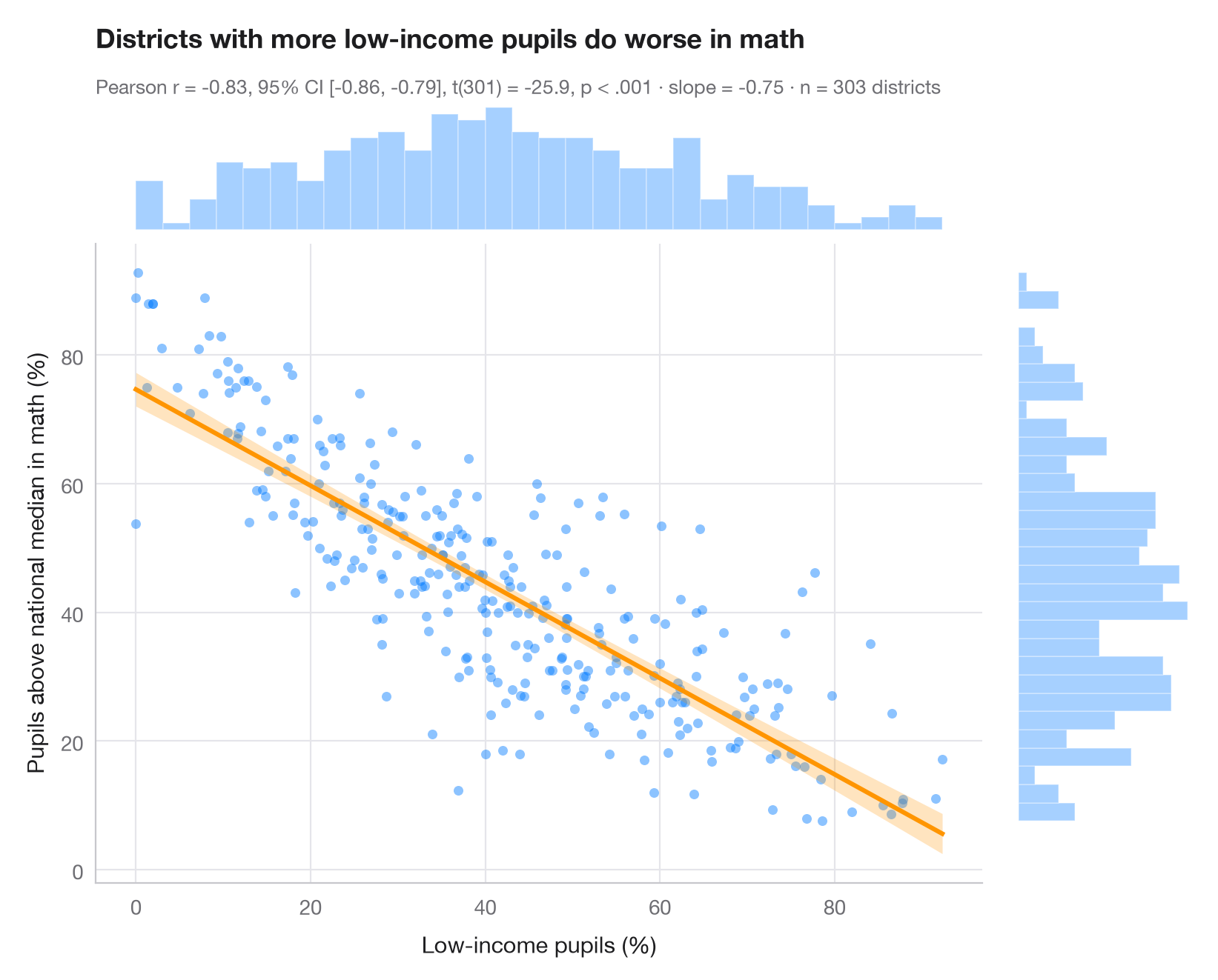
ggscatterstats() の Python 版です。中央のパネルには、すべての観測値と最小二乗直線、およびその 95% 信頼帯(個々の点ではなく、各 x における y の平均についての不確実性)を示しています。上と右の周辺ヒストグラムは各変数の分布の形を示します。相関係数は、この形が妥当であることを暗黙のうちに前提としています。サブタイトルには、ピアソンの r とその 95% 信頼区間、t 検定、OLS の傾き、標本サイズを示しています。
データは statsmodels に同梱されている STAR98 テストのカリフォルニア州 303 学区(sm.datasets.star98)です。低所得世帯の児童の割合と、数学で全国中央値を上回った受験児童の割合(NABOVE / (NABOVE + NBELOW) として計算)を対比しています。傾き −0.75 は、低所得の児童の割合が 10 ポイント高いごとに、中央値を上回る児童の割合が約 7.5 ポイント低いことを意味します。これは学区間の関連であり、効果ではありません。検定は scipy.stats.pearsonr、直線と信頼帯は statsmodels の OLS の get_prediction().conf_int() によるものです。
コードおよび図中のテキストは英語です。
import matplotlib.pyplot as plt
import numpy as np
import statsmodels.api as sm
from scipy import stats

# Data: low-income pupils and math results in 303 California school districts
data = sm.datasets.star98.load_pandas().data
x = data["LOWINC"].to_numpy()
y = (100 * data["NABOVE"] / (data["NABOVE"] + data["NBELOW"])).to_numpy()
n = len(x)

# Pearson correlation with its 95% CI
res = stats.pearsonr(x, y)
ci = res.confidence_interval(0.95)

# OLS fit and 95% confidence band for the mean
fit = sm.OLS(y, sm.add_constant(x)).fit()
grid = np.linspace(x.min(), x.max(), 200)
band = fit.get_prediction(sm.add_constant(grid)).conf_int(alpha=0.05)

fig = plt.figure(figsize=(8, 6.4))
gs = fig.add_gridspec(2, 2, width_ratios=(5, 1), height_ratios=(1, 5), wspace=0.03, hspace=0.03)
ax = fig.add_subplot(gs[1, 0])
ax_top = fig.add_subplot(gs[0, 0], sharex=ax)
ax_right = fig.add_subplot(gs[1, 1], sharey=ax)

ax.scatter(x, y, s=22, color="#007AFF", alpha=0.45, lw=0)
ax.fill_between(grid, band[:, 0], band[:, 1], color="#FF9500", alpha=0.25, lw=0)
ax.plot(grid, fit.params[0] + fit.params[1] * grid, color="#FF9500", lw=2.2)
ax.set_xlabel("Low-income pupils (%)")
ax.set_ylabel("Pupils above national median in math (%)")
ax.grid(axis="x")

# Marginal histograms
ax_top.hist(x, bins=30, color="#007AFF", alpha=0.35, edgecolor="white")
ax_right.hist(y, bins=30, color="#007AFF", alpha=0.35, edgecolor="white", orientation="horizontal")
for a in (ax_top, ax_right):
    a.axis("off")

ax_top.set_title("Districts with more low-income pupils do worse in math", pad=26)
p_txt = "p < .001" if res.pvalue < 0.001 else f"p = {res.pvalue:.3f}"
ax_top.text(0, 1.06, f"Pearson r = {res.statistic:.2f}, 95% CI [{ci.low:.2f}, {ci.high:.2f}], "
            f"t({n - 2}) = {fit.tvalues[1]:.1f}, {p_txt} · slope = {fit.params[1]:.2f} · n = {n} districts",
            transform=ax_top.transAxes, fontsize=9.5, color="#6E6E73")
plt.show()
図にはオプションの PyStatlas スタイル を使用しています。同じ見た目にするには plt.style.use("pystatlas.mplstyle") を追加してください。
データの出典
- California STAR test results, 1998 (303 school districts). Gill, J. (2001). Generalized Linear Models: A Unified Approach (Quantitative Applications in the Social Sciences, No. 134). Sage. https://www.statsmodels.org/stable/datasets/generated/star98.html
Original data from the California Department of Education's Standardized Testing and Reporting (STAR) program, 1998. Subset distributed with statsmodels (sm.datasets.star98) with the author's permission.
これらの例は統計手法を説明するためのものです。図のタイトルは、この特定のデータ(多くは小規模で、古く、部分的な標本)で図が示す内容を述べたものであり、実質的な問いに対する著者の立場ではありません。解釈、背景、データの質については、ここに挙げた元の出典を参照してください。
引用方法
PyStatlas は Thierry Warin が作成・運営しています。研究や業務に役立った場合は、ぜひ引用してください。
Warin, T. (2026). Scatterplot with statistics. In PyStatlas: A Python Gallery of Statistical Graphics for the Social Sciences. https://warint.github.io/pystatlas/correlation/scatter-with-stats/
@misc{warin2026statlas,
  author       = {Warin, Thierry},
  title        = {PyStatlas: A Python Gallery of Statistical Graphics for the Social Sciences},
  year         = {2026},
  howpublished = {\url{https://warint.github.io/pystatlas/}},
  note         = {Source code: https://github.com/warint/pystatlas}
}