附统计量的散点图
加州 303 个学区的低收入学生比例与数学成绩——散点图、附 95% 置信带的 OLS 回归线、边际直方图和 Pearson r。
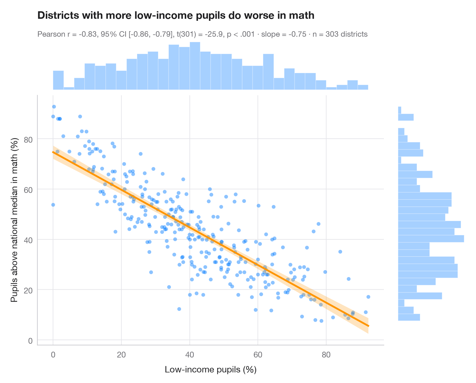
ggscatterstats() 的 Python 版本。中央面板展示所有观测值,以及最小二乘回归线和其 95% 置信带(反映的是每个 x 处 y 均值的不确定性,而非单个数据点的不确定性)。上方和右侧的边际直方图揭示了每个变量的分布形态——相关系数默认这一形态是合理的。副标题报告 Pearson r 及其 95% 置信区间、t 检验、OLS 斜率和样本量。
数据为 statsmodels 自带的 STAR98 测试中加州 303 个学区(sm.datasets.star98):低收入家庭学生的比例,对比数学成绩高于全国中位数的受测学生比例,后者按 NABOVE / (NABOVE + NBELOW) 计算。斜率 −0.75 意味着低收入学生比例每高 10 个百分点,高于中位数的学生比例约低 7.5 个百分点——这是学区之间的关联,而非因果效应。检验来自 scipy.stats.pearsonr,回归线和置信带来自 statsmodels OLS 的 get_prediction().conf_int()。
代码及图中文字均为英文。
import matplotlib.pyplot as plt
import numpy as np
import statsmodels.api as sm
from scipy import stats

# Data: low-income pupils and math results in 303 California school districts
data = sm.datasets.star98.load_pandas().data
x = data["LOWINC"].to_numpy()
y = (100 * data["NABOVE"] / (data["NABOVE"] + data["NBELOW"])).to_numpy()
n = len(x)

# Pearson correlation with its 95% CI
res = stats.pearsonr(x, y)
ci = res.confidence_interval(0.95)

# OLS fit and 95% confidence band for the mean
fit = sm.OLS(y, sm.add_constant(x)).fit()
grid = np.linspace(x.min(), x.max(), 200)
band = fit.get_prediction(sm.add_constant(grid)).conf_int(alpha=0.05)

fig = plt.figure(figsize=(8, 6.4))
gs = fig.add_gridspec(2, 2, width_ratios=(5, 1), height_ratios=(1, 5), wspace=0.03, hspace=0.03)
ax = fig.add_subplot(gs[1, 0])
ax_top = fig.add_subplot(gs[0, 0], sharex=ax)
ax_right = fig.add_subplot(gs[1, 1], sharey=ax)

ax.scatter(x, y, s=22, color="#007AFF", alpha=0.45, lw=0)
ax.fill_between(grid, band[:, 0], band[:, 1], color="#FF9500", alpha=0.25, lw=0)
ax.plot(grid, fit.params[0] + fit.params[1] * grid, color="#FF9500", lw=2.2)
ax.set_xlabel("Low-income pupils (%)")
ax.set_ylabel("Pupils above national median in math (%)")
ax.grid(axis="x")

# Marginal histograms
ax_top.hist(x, bins=30, color="#007AFF", alpha=0.35, edgecolor="white")
ax_right.hist(y, bins=30, color="#007AFF", alpha=0.35, edgecolor="white", orientation="horizontal")
for a in (ax_top, ax_right):
    a.axis("off")

ax_top.set_title("Districts with more low-income pupils do worse in math", pad=26)
p_txt = "p < .001" if res.pvalue < 0.001 else f"p = {res.pvalue:.3f}"
ax_top.text(0, 1.06, f"Pearson r = {res.statistic:.2f}, 95% CI [{ci.low:.2f}, {ci.high:.2f}], "
            f"t({n - 2}) = {fit.tvalues[1]:.1f}, {p_txt} · slope = {fit.params[1]:.2f} · n = {n} districts",
            transform=ax_top.transAxes, fontsize=9.5, color="#6E6E73")
plt.show()
图表使用了可选的 PyStatlas 样式:添加 plt.style.use("pystatlas.mplstyle") 即可完全还原其外观。
数据来源
- California STAR test results, 1998 (303 school districts). Gill, J. (2001). Generalized Linear Models: A Unified Approach (Quantitative Applications in the Social Sciences, No. 134). Sage. https://www.statsmodels.org/stable/datasets/generated/star98.html
Original data from the California Department of Education's Standardized Testing and Reporting (STAR) program, 1998. Subset distributed with statsmodels (sm.datasets.star98) with the author's permission.
这些示例用于说明统计方法。图表标题描述的是该图在这些特定数据中呈现的内容——这些数据往往样本较小、年代较早或并不完整——而不是作者对实质问题的立场。关于解释、背景和数据质量,请以此处引用的原始来源为准。
如何引用
PyStatlas 由 Thierry Warin 创建并维护。如果它对你的工作有所帮助,敬请引用。
Warin, T. (2026). Scatterplot with statistics. In PyStatlas: A Python Gallery of Statistical Graphics for the Social Sciences. https://warint.github.io/pystatlas/correlation/scatter-with-stats/
@misc{warin2026statlas,
  author       = {Warin, Thierry},
  title        = {PyStatlas: A Python Gallery of Statistical Graphics for the Social Sciences},
  year         = {2026},
  howpublished = {\url{https://warint.github.io/pystatlas/}},
  note         = {Source code: https://github.com/warint/pystatlas}
}