相关矩阵
下三角 Pearson 相关热图;不显著的单元格(Holm 校正)以叉号划去。
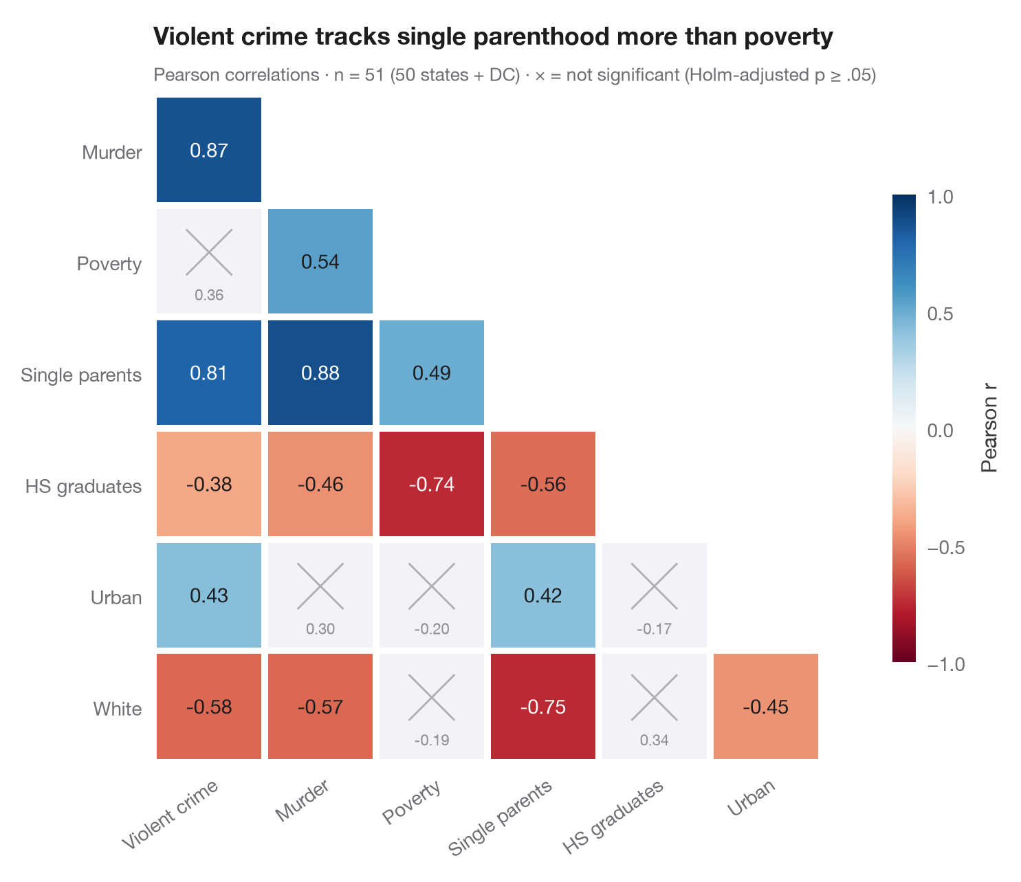
ggcorrmat() 的 Python 版本。由于相关矩阵是对称的,只绘制下三角;每个色块显示 Pearson r,并以从 −1(红)到 +1(蓝)的发散色阶着色。因为同时检验了 21 个相关系数,p 值经过 Holm 校正,校正后在 α = .05 水平上不显著的变量对会变灰并打叉,视线可以直接略过。
数据为 statsmodels 自带的美国各州犯罪统计(sm.datasets.statecrime,50 个州 + 哥伦比亚特区)。相关系数和 p 值由 scipy.stats.pearsonr 计算,校正由 statsmodels.stats.multitest.multipletests(method="holm") 完成。
代码及图中文字均为英文。
from itertools import combinations

import matplotlib.pyplot as plt
import numpy as np
import statsmodels.api as sm
from scipy import stats
from statsmodels.stats.multitest import multipletests

# Data: US state crime statistics (bundled with statsmodels)
df = sm.datasets.statecrime.load_pandas().data
names = {"violent": "Violent crime", "murder": "Murder", "poverty": "Poverty",
         "single": "Single parents", "hs_grad": "HS graduates", "urban": "Urban", "white": "White"}
df = df[list(names)].rename(columns=names)
k = df.shape[1]

# Pearson r and Holm-adjusted p-values for every pair
pairs = list(combinations(range(k), 2))
tests = [stats.pearsonr(df.iloc[:, i], df.iloc[:, j]) for i, j in pairs]
p_adj = multipletests([t.pvalue for t in tests], method="holm")[1]

fig, ax = plt.subplots(figsize=(7.6, 6.2))
cmap, norm = plt.get_cmap("RdBu"), plt.Normalize(-1, 1)
for (i, j), t, p in zip(pairs, tests, p_adj):
    row, col = j, i                                    # lower triangle: row > column
    sig = p < 0.05
    ax.add_patch(plt.Rectangle((col - 0.5 + 0.03, row - 0.5 + 0.03), 0.94, 0.94,
                               color=cmap(norm(t.statistic)) if sig else "#F2F2F7", lw=0))
    if sig:
        ax.text(col, row, f"{t.statistic:.2f}", ha="center", va="center", fontsize=10.5,
                color="white" if abs(t.statistic) > 0.6 else "#1D1D1F")
    else:
        ax.plot([col - 0.2, col + 0.2], [row - 0.28, row + 0.12], color="#AEAEB2", lw=1)
        ax.plot([col - 0.2, col + 0.2], [row + 0.12, row - 0.28], color="#AEAEB2", lw=1)
        ax.text(col, row + 0.3, f"{t.statistic:.2f}", ha="center", va="center", fontsize=8, color="#8E8E93")

ax.set_xlim(-0.5, k - 1.5)
ax.set_ylim(k - 0.5, 0.5)
ax.set_xticks(range(k - 1), df.columns[:-1], rotation=35, ha="right", rotation_mode="anchor")
ax.set_yticks(range(1, k), df.columns[1:])
ax.set_aspect("equal")
ax.grid(False)
for s in ax.spines.values():
    s.set_visible(False)

cb = fig.colorbar(plt.cm.ScalarMappable(norm=norm, cmap=cmap), ax=ax, shrink=0.7, pad=0.02,
                  ticks=[-1, -0.5, 0, 0.5, 1])
cb.set_label("Pearson r", color="#3A3A3C")
cb.outline.set_visible(False)
ax.set_title("Violent crime tracks single parenthood more than poverty", pad=26)
ax.text(0, 1.02, f"Pearson correlations · n = {len(df)} (50 states + DC) · "
        f"× = not significant (Holm-adjusted p ≥ .05)", transform=ax.transAxes,
        fontsize=9.5, color="#6E6E73")
plt.show()
图表使用了可选的 PyStatlas 样式:添加 plt.style.use("pystatlas.mplstyle") 即可完全还原其外观。
数据来源
- US state crime and social indicators, 2009. U.S. Census Bureau. Statistical Abstract of the United States, state tables for 2009 (crime rates from the FBI Uniform Crime Reporting program). https://www.statsmodels.org/stable/datasets/generated/statecrime.html
Compiled for statsmodels (sm.datasets.statecrime); public domain. See the statsmodels page for each variable's table and footnotes.
这些示例用于说明统计方法。图表标题描述的是该图在这些特定数据中呈现的内容——这些数据往往样本较小、年代较早或并不完整——而不是作者对实质问题的立场。关于解释、背景和数据质量,请以此处引用的原始来源为准。
如何引用
PyStatlas 由 Thierry Warin 创建并维护。如果它对你的工作有所帮助,敬请引用。
Warin, T. (2026). Correlation matrix. In PyStatlas: A Python Gallery of Statistical Graphics for the Social Sciences. https://warint.github.io/pystatlas/correlation/correlation-matrix/
@misc{warin2026statlas,
  author       = {Warin, Thierry},
  title        = {PyStatlas: A Python Gallery of Statistical Graphics for the Social Sciences},
  year         = {2026},
  howpublished = {\url{https://warint.github.io/pystatlas/}},
  note         = {Source code: https://github.com/warint/pystatlas}
}