クラスタリング付きコレログラム
学区に関する 13 の指標について、r に応じて大きさと色を決めた corrplot 風の円を、階層的クラスタリングの順に並べたものです。
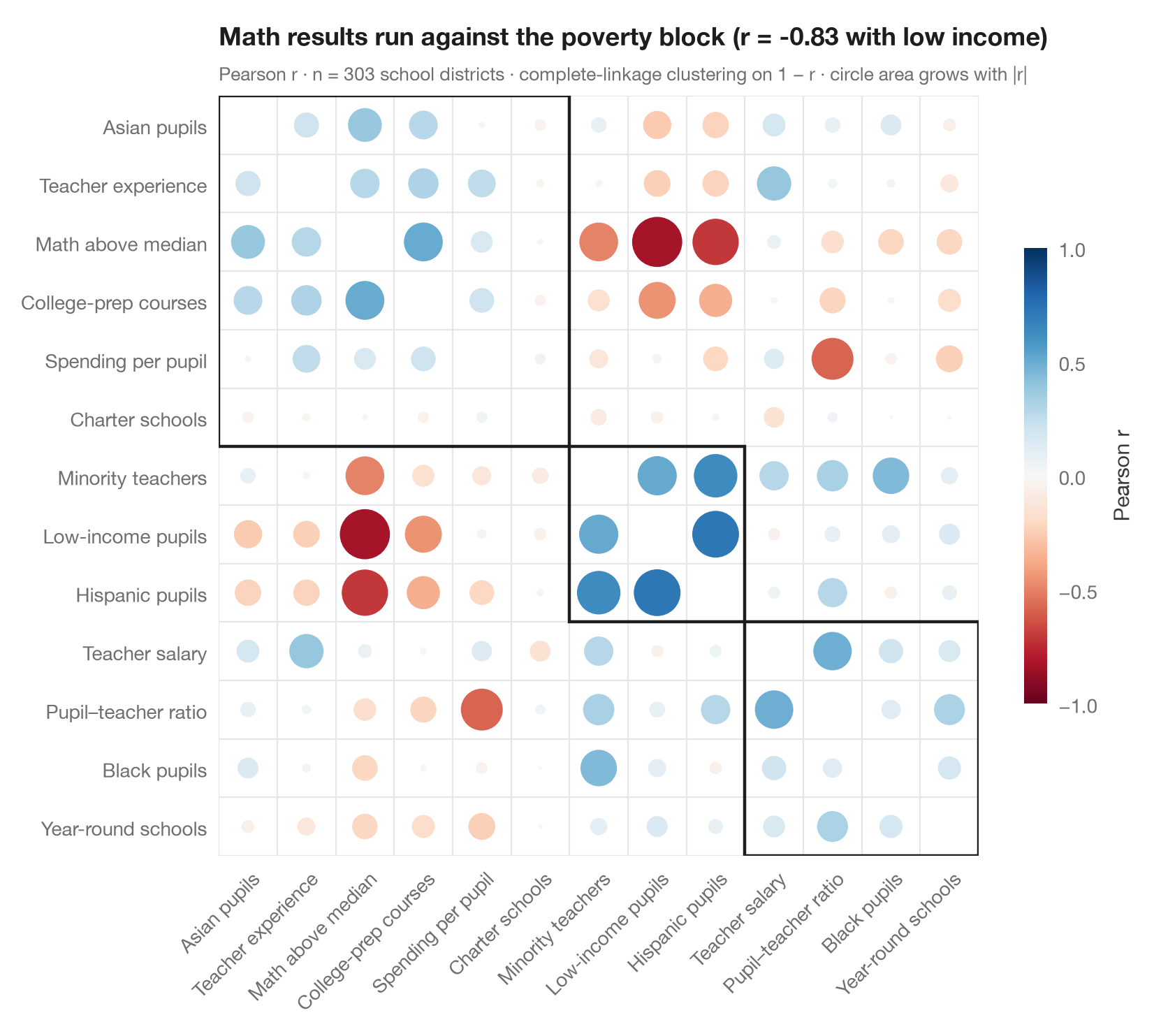
corrplot(method = "circle", order = "hclust") の Python 版です。各円の 面積 は |r| とともに大きくなり、色は符号を表すため、強い相関は目立ち、弱い相関は薄れて見えます。変数は 階層的クラスタリング(距離 1 − r に対する完全連結法)によって並べ替えられ、正の相関をもつ変数どうしが対角線に沿ってブロックにまとまります。枠は addrect = 3 と同様に3つのクラスターを囲んでいます。ここでは低所得の児童、ヒスパニック系の児童、マイノリティの教員が一つのブロックを成し、数学の成績はその 3 つすべてと負の相関を示します。
データは statsmodels に同梱されている STAR98 テストのカリフォルニア州 303 学区(sm.datasets.star98)に関する 13 の指標です。数学の成績(全国中央値を上回る児童の割合)、児童の構成(低所得、ヒスパニック系、黒人、アジア系の児童)、教員(マイノリティの割合、経験年数、給与)、資源(児童一人当たり支出、児童・教員比)、学校の編成(大学進学準備コース、チャータースクール、通年制の学校)を含みます。並び順は scipy.cluster.hierarchy.linkage と leaves_list、枠は fcluster によるものです。
コードおよび図中のテキストは英語です。
import matplotlib.pyplot as plt
import numpy as np
import statsmodels.api as sm
from matplotlib.patches import Circle, Rectangle
from scipy.cluster.hierarchy import fcluster, leaves_list, linkage
from scipy.spatial.distance import squareform

# Data: 13 indicators for 303 California school districts (STAR98, bundled with statsmodels)
df = sm.datasets.star98.load_pandas().data
df["MATH"] = 100 * df.NABOVE / (df.NABOVE + df.NBELOW)
labels = {"MATH": "Math above median", "LOWINC": "Low-income pupils",
          "PERHISP": "Hispanic pupils", "PERBLACK": "Black pupils",
          "PERASIAN": "Asian pupils", "PERMINTE": "Minority teachers",
          "AVYRSEXP": "Teacher experience", "AVSALK": "Teacher salary",
          "PERSPENK": "Spending per pupil", "PTRATIO": "Pupil–teacher ratio",
          "PCTAF": "College-prep courses", "PCTCHRT": "Charter schools",
          "PCTYRRND": "Year-round schools"}
df = df[list(labels)].rename(columns=labels)
corr = df.corr()

# Hierarchical clustering on the distance 1 - r, then reorder the matrix
Z = linkage(squareform(1 - corr.to_numpy(), checks=False), method="complete")
order = leaves_list(Z)
corr = corr.iloc[order, order]
clusters = fcluster(Z, t=3, criterion="maxclust")[order]
k = len(corr)

fig, ax = plt.subplots(figsize=(8.4, 7.2))
cmap, norm = plt.get_cmap("RdBu"), plt.Normalize(-1, 1)
for i in range(k):
    for j in range(k):
        r = corr.iat[i, j]
        if i == j:
            continue
        ax.add_patch(Circle((j, i), radius=0.47 * np.sqrt(abs(r)), color=cmap(norm(r)), lw=0))

# Boxes around the clusters (consecutive runs along the diagonal)
start = 0
for idx in range(1, k + 1):
    if idx == k or clusters[idx] != clusters[start]:
        ax.add_patch(Rectangle((start - 0.5, start - 0.5), idx - start, idx - start,
                               fill=False, ec="#1D1D1F", lw=1.6))
        start = idx

ax.set_xticks(range(k), corr.columns, rotation=45, ha="right", rotation_mode="anchor")
ax.set_yticks(range(k), corr.index)
ax.set_xticks(np.arange(-0.5, k), minor=True)
ax.set_yticks(np.arange(-0.5, k), minor=True)
ax.grid(which="minor", color="#E5E5EA", lw=0.8)
ax.grid(which="major", visible=False)
ax.tick_params(which="minor", length=0)
ax.set_xlim(-0.5, k - 0.5)
ax.set_ylim(k - 0.5, -0.5)
ax.set_aspect("equal")
for s in ax.spines.values():
    s.set_visible(False)

cb = fig.colorbar(plt.cm.ScalarMappable(norm=norm, cmap=cmap), ax=ax, shrink=0.6, pad=0.02,
                  ticks=[-1, -0.5, 0, 0.5, 1])
cb.set_label("Pearson r", color="#3A3A3C")
cb.outline.set_visible(False)
r_pov = corr.loc["Math above median", "Low-income pupils"]
ax.set_title(f"Math results run against the poverty block (r = {r_pov:.2f} with low income)", pad=26)
ax.text(0, 1.02, f"Pearson r · n = {len(df)} school districts · complete-linkage clustering on 1 − r · "
        "circle area grows with |r|", transform=ax.transAxes, fontsize=9.5, color="#6E6E73")
plt.show()
図にはオプションの PyStatlas スタイル を使用しています。同じ見た目にするには plt.style.use("pystatlas.mplstyle") を追加してください。
データの出典
- California STAR test results, 1998 (303 school districts). Gill, J. (2001). Generalized Linear Models: A Unified Approach (Quantitative Applications in the Social Sciences, No. 134). Sage. https://www.statsmodels.org/stable/datasets/generated/star98.html
Original data from the California Department of Education's Standardized Testing and Reporting (STAR) program, 1998. Subset distributed with statsmodels (sm.datasets.star98) with the author's permission.
これらの例は統計手法を説明するためのものです。図のタイトルは、この特定のデータ(多くは小規模で、古く、部分的な標本)で図が示す内容を述べたものであり、実質的な問いに対する著者の立場ではありません。解釈、背景、データの質については、ここに挙げた元の出典を参照してください。
引用方法
PyStatlas は Thierry Warin が作成・運営しています。研究や業務に役立った場合は、ぜひ引用してください。
Warin, T. (2026). Correlogram with clustering. In PyStatlas: A Python Gallery of Statistical Graphics for the Social Sciences. https://warint.github.io/pystatlas/correlation/correlogram-bubble/
@misc{warin2026statlas,
  author       = {Warin, Thierry},
  title        = {PyStatlas: A Python Gallery of Statistical Graphics for the Social Sciences},
  year         = {2026},
  howpublished = {\url{https://warint.github.io/pystatlas/}},
  note         = {Source code: https://github.com/warint/pystatlas}
}