Kaplan–Meier curves
How long political leaders stay in office, democracies vs non-democracies — survival curves with confidence bands, censoring marks, log-rank test and risk table.
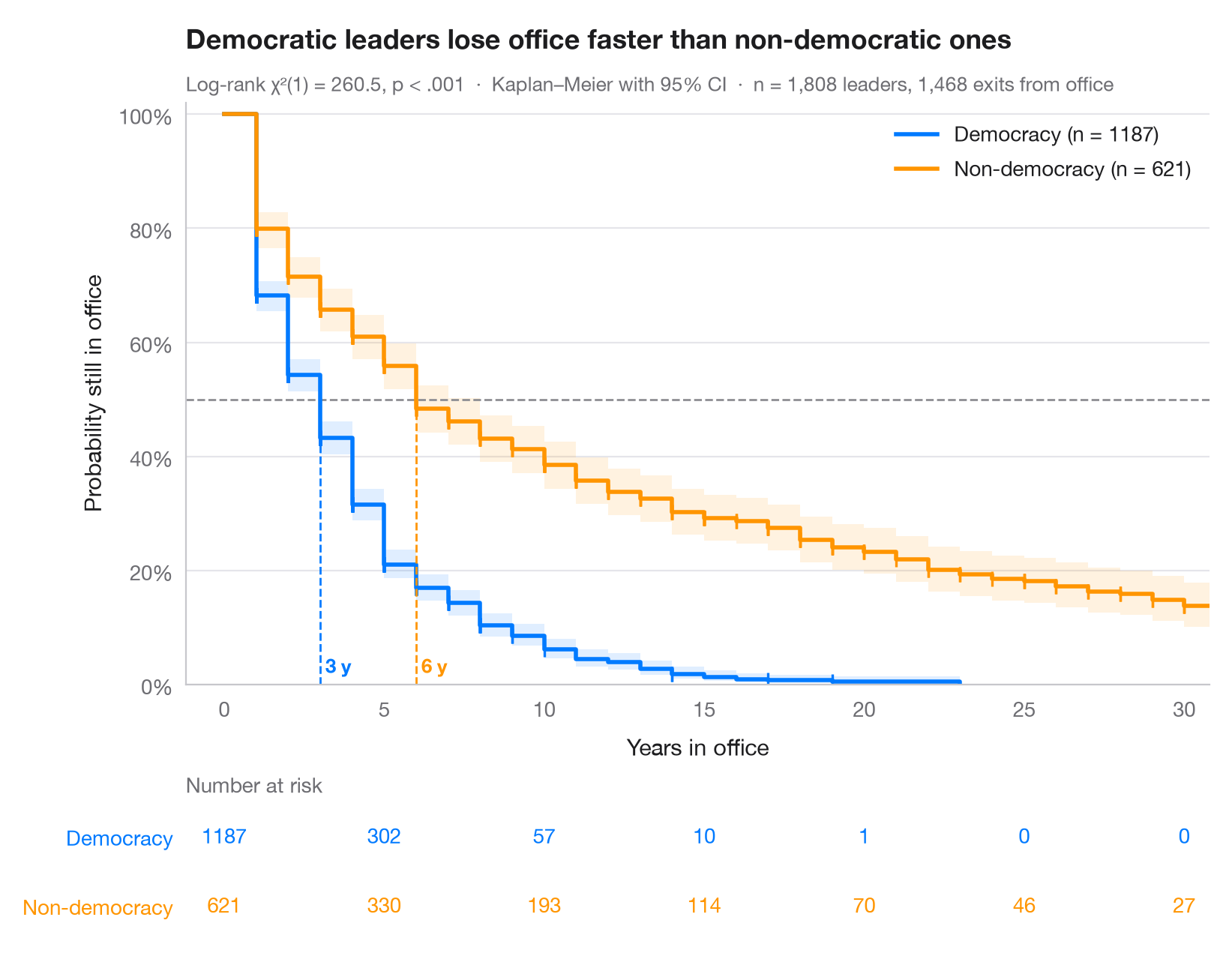
The Kaplan–Meier estimator turns follow-up times — some ending in an event, some censored — into a step curve of the probability of "surviving" beyond each time. Shaded bands are pointwise 95% confidence intervals, small ticks mark censored spells, and dashed lines drop from 50% to the median survival of each group. The table underneath gives the number still at risk, which tells you how much data supports the tail of each curve.
Data are the Democracy and Dictatorship dataset of Cheibub, Gandhi & Vreeland
bundled with lifelines (lifelines.datasets.load_dd): 1,808 spells in
office of heads of government in 202 countries, 1946–2008, timed in years.
The event is leaving office; spells without an observed exit — for instance
those still running when the data end — are censored. Democratic leaders reach
their median tenure twice as fast as non-democratic ones. The x-axis stops at
30 years; no democratic spell lasts beyond 23. Curves come from
KaplanMeierFitter, the comparison from logrank_test.
import matplotlib.pyplot as plt
import numpy as np
from lifelines import KaplanMeierFitter
from lifelines.datasets import load_dd
from lifelines.statistics import logrank_test

# Data: years in office of 1,808 political leaders, by regime type
df = load_dd()
groups = {"Democracy": df[df.democracy == "Democracy"],
          "Non-democracy": df[df.democracy == "Non-democracy"]}
colors = ["#007AFF", "#FF9500"]
ticks = np.arange(0, 31, 5)

fig, (ax, tab) = plt.subplots(2, 1, figsize=(8, 6.2), sharex=True,
                              gridspec_kw=dict(height_ratios=[4.2, 1]))

# Kaplan–Meier fit per group: step curve, CI band, censoring ticks, median line
for (name, d), c in zip(groups.items(), colors):
    km = KaplanMeierFitter().fit(d.duration, d.observed, label=name)
    sf, ci = km.survival_function_[name], km.confidence_interval_
    ax.step(sf.index, sf, where="post", color=c, lw=2, label=f"{name} (n = {len(d)})")
    ax.fill_between(ci.index, ci.iloc[:, 0], ci.iloc[:, 1], step="post", color=c, alpha=0.12, lw=0)
    cens = d.loc[d.observed == 0, "duration"]
    ax.plot(cens, km.survival_function_at_times(cens), "|", color=c, ms=7, mew=1.2)
    med = km.median_survival_time_
    ax.plot([med, med], [0, 0.5], ls="--", lw=1, color=c)
    ax.text(med, 0.02, f" {med:.0f} y", color=c, fontsize=9.5, fontweight="semibold", ha="left")
    # Number at risk under the plot
    at_risk = [(d.duration >= t).sum() for t in ticks]
    for t, n in zip(ticks, at_risk):
        tab.text(t, 1 - list(groups).index(name), n, ha="center", va="center", color=c, fontsize=10)

ax.axhline(0.5, color="#8E8E93", lw=1, ls="--", zorder=1)
ax.set(ylim=(0, 1.02), xlim=(-1.2, 30.8), ylabel="Probability still in office", xlabel="Years in office")
ax.tick_params(labelbottom=True)
ax.yaxis.set_major_formatter(plt.matplotlib.ticker.PercentFormatter(1))
ax.legend(loc="upper right")

# Log-rank test
dem, non = groups["Democracy"], groups["Non-democracy"]
lr = logrank_test(dem.duration, non.duration, dem.observed, non.observed)
p_txt = "p < .001" if lr.p_value < 0.001 else f"p = {lr.p_value:.3f}"
ax.set_title("Democratic leaders lose office faster than non-democratic ones", pad=26)
ax.text(0, 1.02, f"Log-rank χ²(1) = {lr.test_statistic:.1f}, {p_txt}  ·  "
        f"Kaplan–Meier with 95% CI  ·  n = {len(df):,} leaders, {df.observed.sum():,} exits from office",
        transform=ax.transAxes, fontsize=9.5, color="#6E6E73")

# Risk table styling
tab.set(ylim=(-0.5, 1.5), xticks=ticks)
tab.tick_params(labelbottom=False)
tab.set_yticks([1, 0], list(groups))
for lbl, c in zip(tab.get_yticklabels(), colors):
    lbl.set_color(c)
tab.grid(False)
tab.spines[["left", "bottom"]].set_visible(False)
tab.set_title("Number at risk", fontsize=10, fontweight="normal", color="#6E6E73", pad=4)
plt.show()
Figures use the optional PyStatlas style: add plt.style.use("pystatlas.mplstyle") to match the look exactly.
Data source
- Democracy and Dictatorship: leader spells, 1946–2008. Cheibub, J. A., Gandhi, J., & Vreeland, J. R. (2010). Democracy and dictatorship revisited. Public Choice, 143(1–2), 67–101. https://doi.org/10.1007/s11127-009-9491-2
202 countries; distributed with lifelines (lifelines.datasets.load_dd).
The examples illustrate statistical methods. Their titles describe what each figure shows in these particular data — often a small, dated or partial sample — not the author's position on the substantive question. For interpretation, context and data quality, rely on the original sources cited here.
How to cite
PyStatlas is created and maintained by Thierry Warin. If it helped your work, please cite it.
Warin, T. (2026). Kaplan–Meier curves. In PyStatlas: A Python Gallery of Statistical Graphics for the Social Sciences. https://warint.github.io/pystatlas/survival/kaplan-meier/
@misc{warin2026statlas,
  author       = {Warin, Thierry},
  title        = {PyStatlas: A Python Gallery of Statistical Graphics for the Social Sciences},
  year         = {2026},
  howpublished = {\url{https://warint.github.io/pystatlas/}},
  note         = {Source code: https://github.com/warint/pystatlas}
}More in Survival analysis
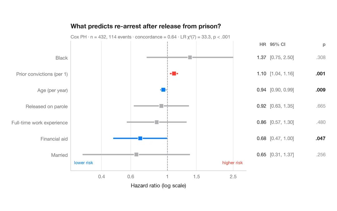
Cox hazard ratios
Forest plot of a Cox proportional hazards model with HR, 95% CI and p-values.
survminer::ggforest()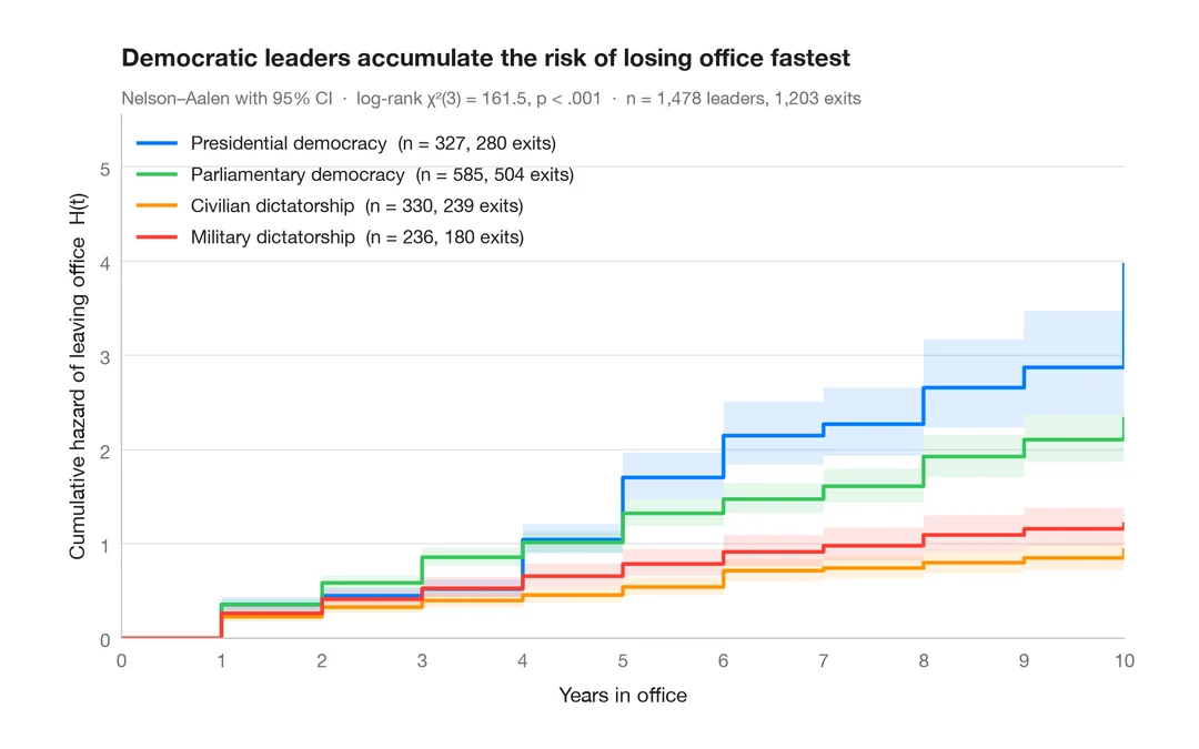
Cumulative hazard
Nelson–Aalen cumulative hazard of leaving office, with 95% bands, for four political regimes.
survminer::ggsurvplot(fun = "cumhaz")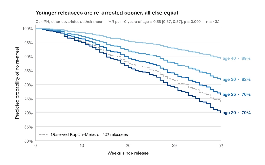
Adjusted survival curves
Cox model–predicted survival for several ages, other covariates held at their mean.
survminer::ggadjustedcurves()