カプラン・マイヤー曲線
政治指導者が在任し続ける期間、民主制と非民主制の比較 — 信頼帯、打ち切りの印、ログランク検定、リスク集合の表付きの生存曲線。
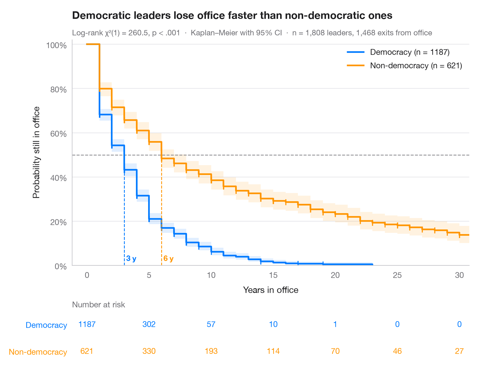
カプラン・マイヤー推定量は、追跡期間(イベントで終わるものもあれば、打ち切りとなるものもあります)を、各時点を超えて「生存」する確率を表す階段状の曲線に変換します。網掛けの帯は各時点ごとの 95% 信頼区間、小さな目盛りは打ち切りとなった在任期間を示し、破線は 50% から各群の 生存期間中央値 へと下ろしています。下の表はまだリスクにさらされている数を示しており、各曲線の裾がどれだけのデータに支えられているかがわかります。
データは lifelines に同梱されている Cheibub, Gandhi & Vreeland の Democracy and Dictatorship データセット(lifelines.datasets.load_dd)で、1946–2008 年の 202 か国における政府首脳の在任期間 1,808 件を年単位で記録しています。イベントは退任であり、退任が観測されていない在任期間(たとえばデータの終了時点でまだ続いていたもの)は打ち切りとして扱います。民主制の指導者は、非民主制の指導者の半分の期間で在任期間の中央値に達します。横軸は 30 年で止めています。民主制の在任期間で 23 年を超えるものはありません。曲線は KaplanMeierFitter、比較は logrank_test によるものです。
コードおよび図中のテキストは英語です。
import matplotlib.pyplot as plt
import numpy as np
from lifelines import KaplanMeierFitter
from lifelines.datasets import load_dd
from lifelines.statistics import logrank_test

# Data: years in office of 1,808 political leaders, by regime type
df = load_dd()
groups = {"Democracy": df[df.democracy == "Democracy"],
          "Non-democracy": df[df.democracy == "Non-democracy"]}
colors = ["#007AFF", "#FF9500"]
ticks = np.arange(0, 31, 5)

fig, (ax, tab) = plt.subplots(2, 1, figsize=(8, 6.2), sharex=True,
                              gridspec_kw=dict(height_ratios=[4.2, 1]))

# Kaplan–Meier fit per group: step curve, CI band, censoring ticks, median line
for (name, d), c in zip(groups.items(), colors):
    km = KaplanMeierFitter().fit(d.duration, d.observed, label=name)
    sf, ci = km.survival_function_[name], km.confidence_interval_
    ax.step(sf.index, sf, where="post", color=c, lw=2, label=f"{name} (n = {len(d)})")
    ax.fill_between(ci.index, ci.iloc[:, 0], ci.iloc[:, 1], step="post", color=c, alpha=0.12, lw=0)
    cens = d.loc[d.observed == 0, "duration"]
    ax.plot(cens, km.survival_function_at_times(cens), "|", color=c, ms=7, mew=1.2)
    med = km.median_survival_time_
    ax.plot([med, med], [0, 0.5], ls="--", lw=1, color=c)
    ax.text(med, 0.02, f" {med:.0f} y", color=c, fontsize=9.5, fontweight="semibold", ha="left")
    # Number at risk under the plot
    at_risk = [(d.duration >= t).sum() for t in ticks]
    for t, n in zip(ticks, at_risk):
        tab.text(t, 1 - list(groups).index(name), n, ha="center", va="center", color=c, fontsize=10)

ax.axhline(0.5, color="#8E8E93", lw=1, ls="--", zorder=1)
ax.set(ylim=(0, 1.02), xlim=(-1.2, 30.8), ylabel="Probability still in office", xlabel="Years in office")
ax.tick_params(labelbottom=True)
ax.yaxis.set_major_formatter(plt.matplotlib.ticker.PercentFormatter(1))
ax.legend(loc="upper right")

# Log-rank test
dem, non = groups["Democracy"], groups["Non-democracy"]
lr = logrank_test(dem.duration, non.duration, dem.observed, non.observed)
p_txt = "p < .001" if lr.p_value < 0.001 else f"p = {lr.p_value:.3f}"
ax.set_title("Democratic leaders lose office faster than non-democratic ones", pad=26)
ax.text(0, 1.02, f"Log-rank χ²(1) = {lr.test_statistic:.1f}, {p_txt}  ·  "
        f"Kaplan–Meier with 95% CI  ·  n = {len(df):,} leaders, {df.observed.sum():,} exits from office",
        transform=ax.transAxes, fontsize=9.5, color="#6E6E73")

# Risk table styling
tab.set(ylim=(-0.5, 1.5), xticks=ticks)
tab.tick_params(labelbottom=False)
tab.set_yticks([1, 0], list(groups))
for lbl, c in zip(tab.get_yticklabels(), colors):
    lbl.set_color(c)
tab.grid(False)
tab.spines[["left", "bottom"]].set_visible(False)
tab.set_title("Number at risk", fontsize=10, fontweight="normal", color="#6E6E73", pad=4)
plt.show()
図にはオプションの PyStatlas スタイル を使用しています。同じ見た目にするには plt.style.use("pystatlas.mplstyle") を追加してください。
データの出典
- Democracy and Dictatorship: leader spells, 1946–2008. Cheibub, J. A., Gandhi, J., & Vreeland, J. R. (2010). Democracy and dictatorship revisited. Public Choice, 143(1–2), 67–101. https://doi.org/10.1007/s11127-009-9491-2
202 countries; distributed with lifelines (lifelines.datasets.load_dd).
これらの例は統計手法を説明するためのものです。図のタイトルは、この特定のデータ(多くは小規模で、古く、部分的な標本)で図が示す内容を述べたものであり、実質的な問いに対する著者の立場ではありません。解釈、背景、データの質については、ここに挙げた元の出典を参照してください。
引用方法
PyStatlas は Thierry Warin が作成・運営しています。研究や業務に役立った場合は、ぜひ引用してください。
Warin, T. (2026). Kaplan–Meier curves. In PyStatlas: A Python Gallery of Statistical Graphics for the Social Sciences. https://warint.github.io/pystatlas/survival/kaplan-meier/
@misc{warin2026statlas,
  author       = {Warin, Thierry},
  title        = {PyStatlas: A Python Gallery of Statistical Graphics for the Social Sciences},
  year         = {2026},
  howpublished = {\url{https://warint.github.io/pystatlas/}},
  note         = {Source code: https://github.com/warint/pystatlas}
}