Cox モデルのハザード比
HR、95% 信頼区間、p値を示す Cox 比例ハザードモデルのフォレストプロットです。
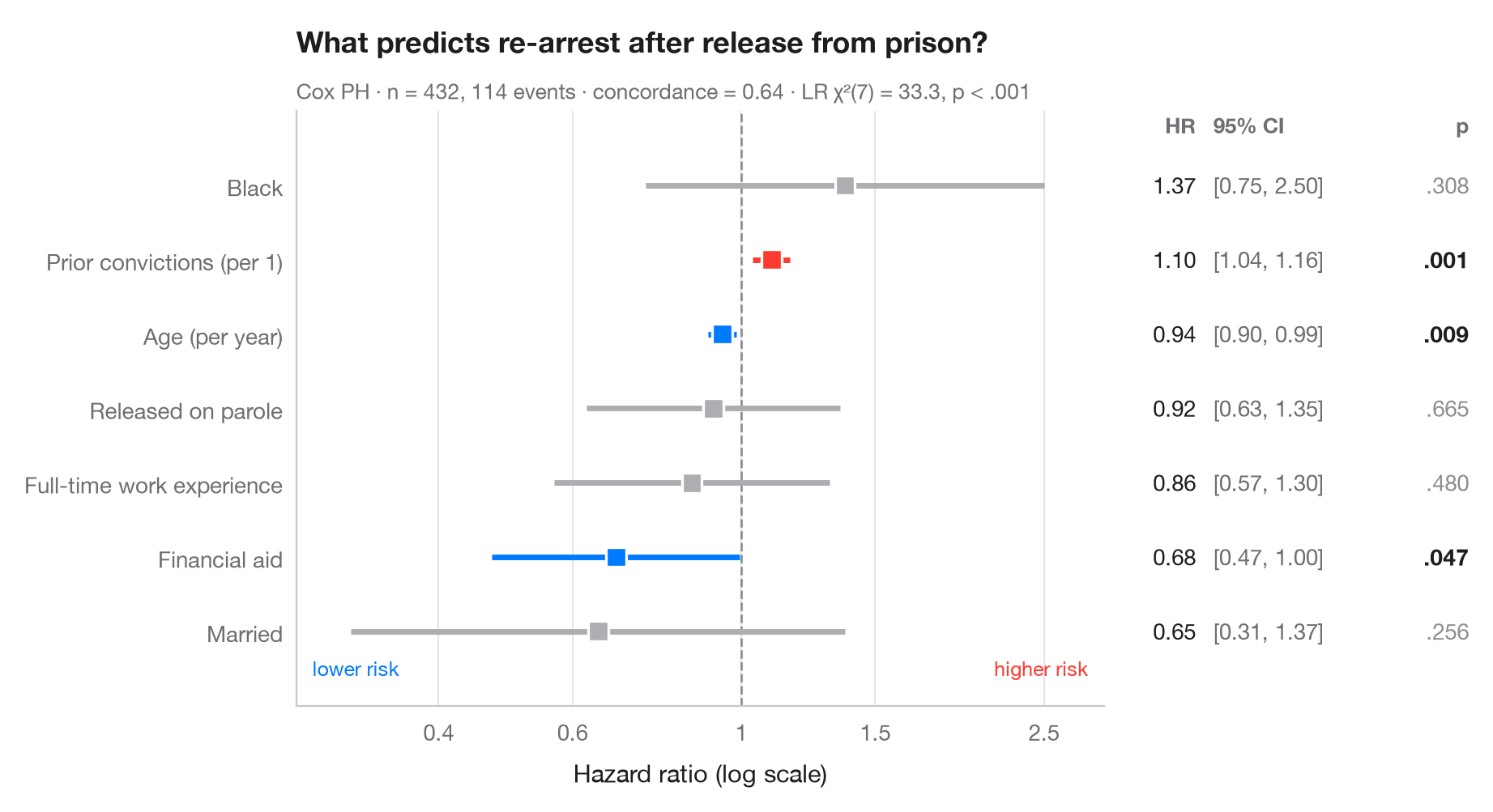
Cox 比例ハザードモデルは、各共変量がイベントの瞬間的なリスクを何倍にするかを推定します。各行は ハザード比(HR)とその 95% 信頼区間を対数スケールで示しているため、リスクが半分になる場合と2倍になる場合は、HR = 1 の基準線から等しい距離に位置します。右側の表には、論文に掲載されるフォレストプロットと同様に数値を再掲しています。
データはロッシの再犯研究(lifelines.datasets.load_rossi)で、釈放された受刑者 432 人を1年間追跡し、再逮捕をイベントとしています。モデルは lifelines.CoxPHFitter で当てはめ、サブタイトルにはコンコーダンス指数とモデル全体の尤度比検定の結果を示しています。
コードおよび図中のテキストは英語です。
import matplotlib.pyplot as plt
import numpy as np
from lifelines import CoxPHFitter
from lifelines.datasets import load_rossi

# Data: weeks to re-arrest after release from prison
df = load_rossi()
cph = CoxPHFitter().fit(df, duration_col="week", event_col="arrest")
lr = cph.log_likelihood_ratio_test()

# Tidy the summary: HR, 95% CI, p-value
labels = {"fin": "Financial aid", "age": "Age (per year)", "race": "Black",
          "wexp": "Full-time work experience", "mar": "Married",
          "paro": "Released on parole", "prio": "Prior convictions (per 1)"}
res = cph.summary.rename(columns={"exp(coef)": "hr", "exp(coef) lower 95%": "low",
                                  "exp(coef) upper 95%": "high"})
res = res.sort_values("hr")
y = np.arange(len(res))
colors = np.where(res.p < 0.05, np.where(res.hr > 1, "#FF3B30", "#007AFF"), "#AEAEB2")

fig, (ax, tab) = plt.subplots(1, 2, figsize=(9, 4.8), sharey=True,
                              gridspec_kw=dict(width_ratios=[3, 1.3]))

# Forest: CI whiskers and point estimates on a log axis
ax.axvline(1, color="#8E8E93", lw=1, ls="--", zorder=1)
ax.hlines(y, res.low, res.high, color=colors, lw=2.5, zorder=2)
ax.scatter(res.hr, y, s=80, marker="s", color=colors, edgecolor="white", lw=1.2, zorder=3)
ax.set_xscale("log")
ax.set_xticks([0.4, 0.6, 1, 1.5, 2.5], ["0.4", "0.6", "1", "1.5", "2.5"])
ax.minorticks_off()
ax.set_xlim(0.26, 3)
ax.set_yticks(y, [labels[t] for t in res.index])
ax.grid(axis="x"); ax.grid(axis="y", visible=False)
ax.set_xlabel("Hazard ratio (log scale)")
ax.text(0.98, -0.6, "higher risk", ha="right", color="#FF3B30", fontsize=9,
        transform=ax.get_yaxis_transform())
ax.text(0.02, -0.6, "lower risk", ha="left", color="#007AFF", fontsize=9,
        transform=ax.get_yaxis_transform())

# Table: HR [95% CI] and p-value
for yi, (_, r) in zip(y, res.iterrows()):
    p = "< .001" if r.p < 0.001 else f"{r.p:.3f}".lstrip("0")
    tab.text(0.22, yi, f"{r.hr:.2f}", va="center", ha="right", fontsize=10, color="#1D1D1F")
    tab.text(0.27, yi, f"[{r.low:.2f}, {r.high:.2f}]", va="center", fontsize=10, color="#6E6E73")
    tab.text(1, yi, p, va="center", ha="right", fontsize=10,
             color="#1D1D1F" if r.p < 0.05 else "#8E8E93",
             fontweight="semibold" if r.p < 0.05 else "normal")
tab.text(0.22, len(res) - 0.3, "HR", ha="right", fontsize=9.5, color="#6E6E73", fontweight="semibold")
tab.text(0.27, len(res) - 0.3, "95% CI", fontsize=9.5, color="#6E6E73", fontweight="semibold")
tab.text(1, len(res) - 0.3, "p", ha="right", fontsize=9.5, color="#6E6E73", fontweight="semibold")
tab.set(xlim=(0, 1), ylim=(-1, len(res)))
tab.axis("off")

ax.set_title("What predicts re-arrest after release from prison?", pad=26)
ax.text(0, 1.02, f"Cox PH · n = {len(df)}, {df.arrest.sum()} events · concordance = "
        f"{cph.concordance_index_:.2f} · LR χ²({lr.degrees_freedom:.0f}) = {lr.test_statistic:.1f}, "
        f"p < .001", transform=ax.transAxes, fontsize=9.5, color="#6E6E73")
plt.show()
図にはオプションの PyStatlas スタイル を使用しています。同じ見た目にするには plt.style.use("pystatlas.mplstyle") を追加してください。
データの出典
- Rossi recidivism experiment (432 released prisoners). Rossi, P. H., Berk, R. A., & Lenihan, K. J. (1980). Money, Work, and Crime: Some Experimental Results. Academic Press. https://lifelines.readthedocs.io/en/latest/lifelines.datasets.html
Men released from Maryland state prisons in the 1970s, half randomly assigned to financial aid. Distributed with lifelines (lifelines.datasets.load_rossi).
これらの例は統計手法を説明するためのものです。図のタイトルは、この特定のデータ(多くは小規模で、古く、部分的な標本)で図が示す内容を述べたものであり、実質的な問いに対する著者の立場ではありません。解釈、背景、データの質については、ここに挙げた元の出典を参照してください。
引用方法
PyStatlas は Thierry Warin が作成・運営しています。研究や業務に役立った場合は、ぜひ引用してください。
Warin, T. (2026). Cox hazard ratios. In PyStatlas: A Python Gallery of Statistical Graphics for the Social Sciences. https://warint.github.io/pystatlas/survival/cox-hazard-ratios/
@misc{warin2026statlas,
  author       = {Warin, Thierry},
  title        = {PyStatlas: A Python Gallery of Statistical Graphics for the Social Sciences},
  year         = {2026},
  howpublished = {\url{https://warint.github.io/pystatlas/}},
  note         = {Source code: https://github.com/warint/pystatlas}
}生存時間分析のその他のグラフ
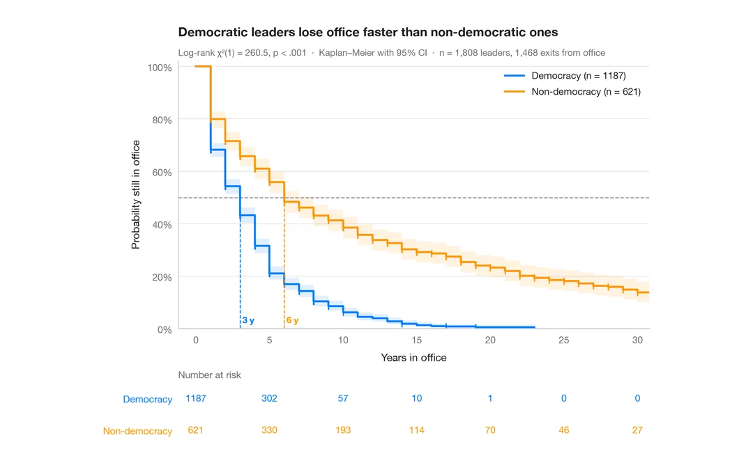
カプラン・マイヤー曲線
政治指導者が在任し続ける期間、民主制と非民主制の比較 — 信頼帯、打ち切りの印、ログランク検定、リスク集合の表付きの生存曲線。
survminer::ggsurvplot(risk.table = TRUE)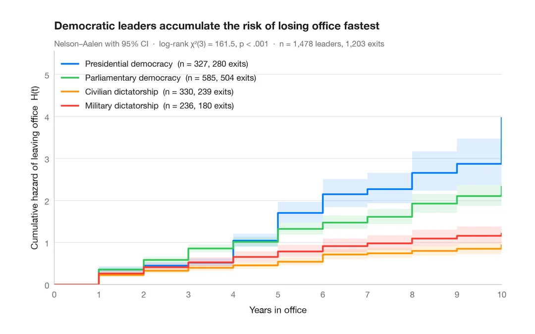
累積ハザード
4 つの政治体制について、退任の Nelson–Aalen 累積ハザードを 95% 信頼帯とともに示します。
survminer::ggsurvplot(fun = "cumhaz")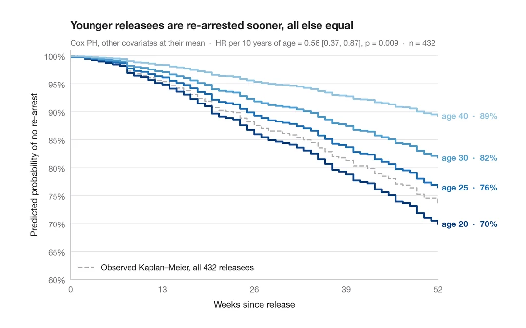
調整済み生存曲線
他の共変量を平均値に固定し、複数の年齢について Cox モデルで予測した生存曲線です。
survminer::ggadjustedcurves()