調整済み生存曲線
他の共変量を平均値に固定し、複数の年齢について Cox モデルで予測した生存曲線です。
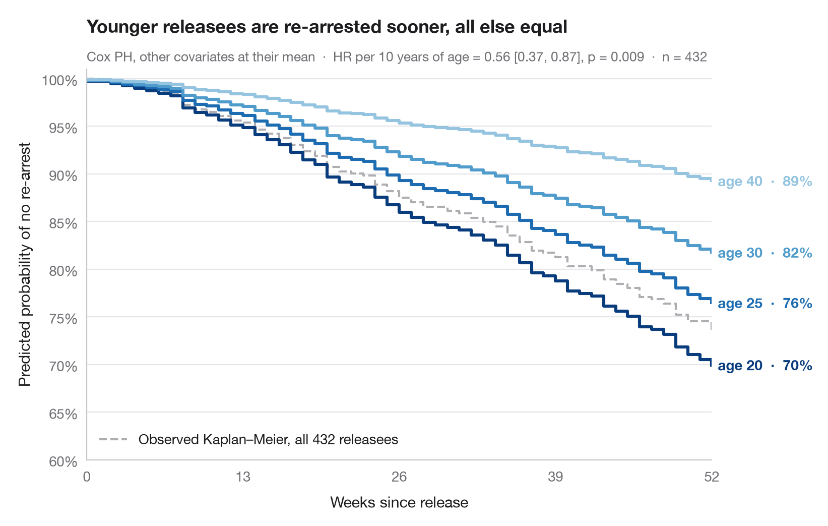
ハザード比は感覚的にとらえにくいものですが、生存曲線ならわかりやすくなります。ここでは当てはめた Cox 比例ハザードモデルを用いて、年齢だけが異なり、他のすべての共変量は標本平均に固定した仮想的な個人について、生存曲線全体を 予測 しています。曲線間の縦方向の開きは、年齢の効果を再逮捕されずにいる確率に置き換えたものです。
データはロッシの再犯研究(lifelines.datasets.load_rossi)です。モデルは7つの共変量すべてを用いて lifelines.CoxPHFitter で当てはめ、曲線は predict_survival_function() から得ています。参考として、標本全体で観測されたカプラン・マイヤー曲線を灰色で描いています。
コードおよび図中のテキストは英語です。
import matplotlib.pyplot as plt
import numpy as np
import pandas as pd
from lifelines import CoxPHFitter, KaplanMeierFitter
from lifelines.datasets import load_rossi

# Data: weeks to re-arrest after release from prison
df = load_rossi()
cph = CoxPHFitter().fit(df, duration_col="week", event_col="arrest")

# Hypothetical profiles: everything at the mean, age varies
ages = [20, 25, 30, 40]
profiles = pd.DataFrame([df.drop(columns=["week", "arrest"]).mean()] * len(ages))
profiles["age"] = ages
surv = cph.predict_survival_function(profiles, times=np.arange(0, 53))
colors = plt.cm.Blues(np.linspace(0.95, 0.4, len(ages)))

fig, ax = plt.subplots(figsize=(8, 5))

# Observed Kaplan–Meier curve of the whole sample, for reference
km = KaplanMeierFitter().fit(df.week, df.arrest)
ax.step(km.survival_function_.index, km.survival_function_.iloc[:, 0], where="post",
        color="#AEAEB2", lw=1.5, ls="--", label=f"Observed Kaplan–Meier, all {len(df)} releasees")
ax.legend(loc="lower left")

# Model-predicted curves, labelled at their end
for col, age, c in zip(surv.columns, ages, colors):
    s = surv[col]
    ax.step(s.index, s, where="post", color=c, lw=2.2)
    ax.text(52.5, s.iloc[-1], f"age {age}  ·  {s.iloc[-1]:.0%}", va="center",
            fontsize=10, color=c, fontweight="semibold")

hr10 = np.exp(10 * cph.params_["age"])
lo, hi = np.exp(10 * cph.confidence_intervals_.loc["age"])
p = cph.summary.loc["age", "p"]
ax.set(xlim=(0, 52), ylim=(0.6, 1.01), xticks=range(0, 53, 13),
       xlabel="Weeks since release", ylabel="Predicted probability of no re-arrest")
ax.yaxis.set_major_formatter(plt.matplotlib.ticker.PercentFormatter(1, decimals=0))
ax.set_title("Younger releasees are re-arrested sooner, all else equal", pad=26)
ax.text(0, 1.02, f"Cox PH, other covariates at their mean  ·  HR per 10 years of age = "
        f"{hr10:.2f} [{lo:.2f}, {hi:.2f}], p = {p:.3f}  ·  n = {len(df)}",
        transform=ax.transAxes, fontsize=9.5, color="#6E6E73")
plt.show()
図にはオプションの PyStatlas スタイル を使用しています。同じ見た目にするには plt.style.use("pystatlas.mplstyle") を追加してください。
データの出典
- Rossi recidivism experiment (432 released prisoners). Rossi, P. H., Berk, R. A., & Lenihan, K. J. (1980). Money, Work, and Crime: Some Experimental Results. Academic Press. https://lifelines.readthedocs.io/en/latest/lifelines.datasets.html
Men released from Maryland state prisons in the 1970s, half randomly assigned to financial aid. Distributed with lifelines (lifelines.datasets.load_rossi).
これらの例は統計手法を説明するためのものです。図のタイトルは、この特定のデータ(多くは小規模で、古く、部分的な標本)で図が示す内容を述べたものであり、実質的な問いに対する著者の立場ではありません。解釈、背景、データの質については、ここに挙げた元の出典を参照してください。
引用方法
PyStatlas は Thierry Warin が作成・運営しています。研究や業務に役立った場合は、ぜひ引用してください。
Warin, T. (2026). Adjusted survival curves. In PyStatlas: A Python Gallery of Statistical Graphics for the Social Sciences. https://warint.github.io/pystatlas/survival/adjusted-survival/
@misc{warin2026statlas,
  author       = {Warin, Thierry},
  title        = {PyStatlas: A Python Gallery of Statistical Graphics for the Social Sciences},
  year         = {2026},
  howpublished = {\url{https://warint.github.io/pystatlas/}},
  note         = {Source code: https://github.com/warint/pystatlas}
}生存時間分析のその他のグラフ
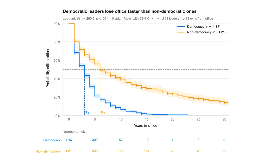
カプラン・マイヤー曲線
政治指導者が在任し続ける期間、民主制と非民主制の比較 — 信頼帯、打ち切りの印、ログランク検定、リスク集合の表付きの生存曲線。
survminer::ggsurvplot(risk.table = TRUE)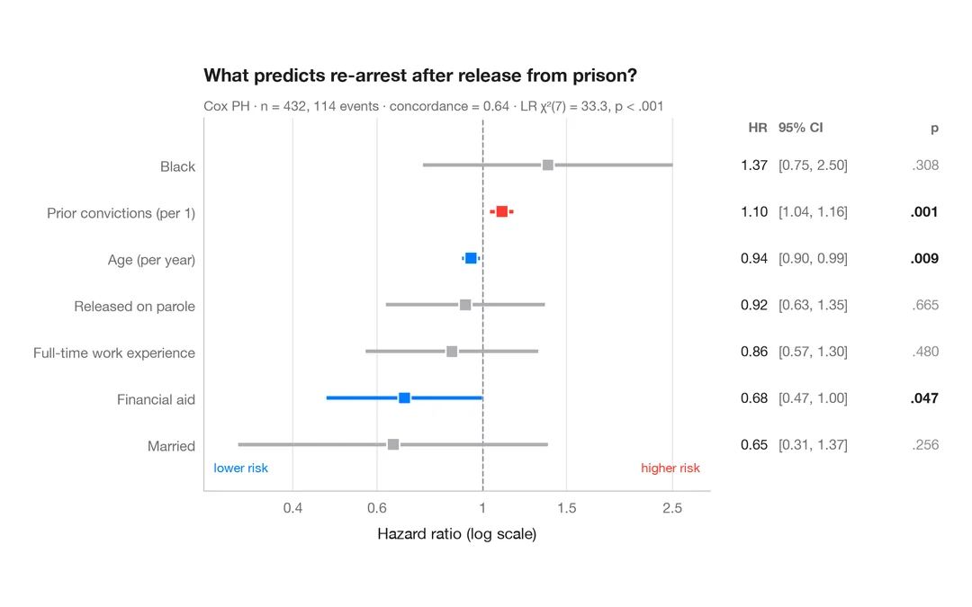
Cox モデルのハザード比
HR、95% 信頼区間、p値を示す Cox 比例ハザードモデルのフォレストプロットです。
survminer::ggforest()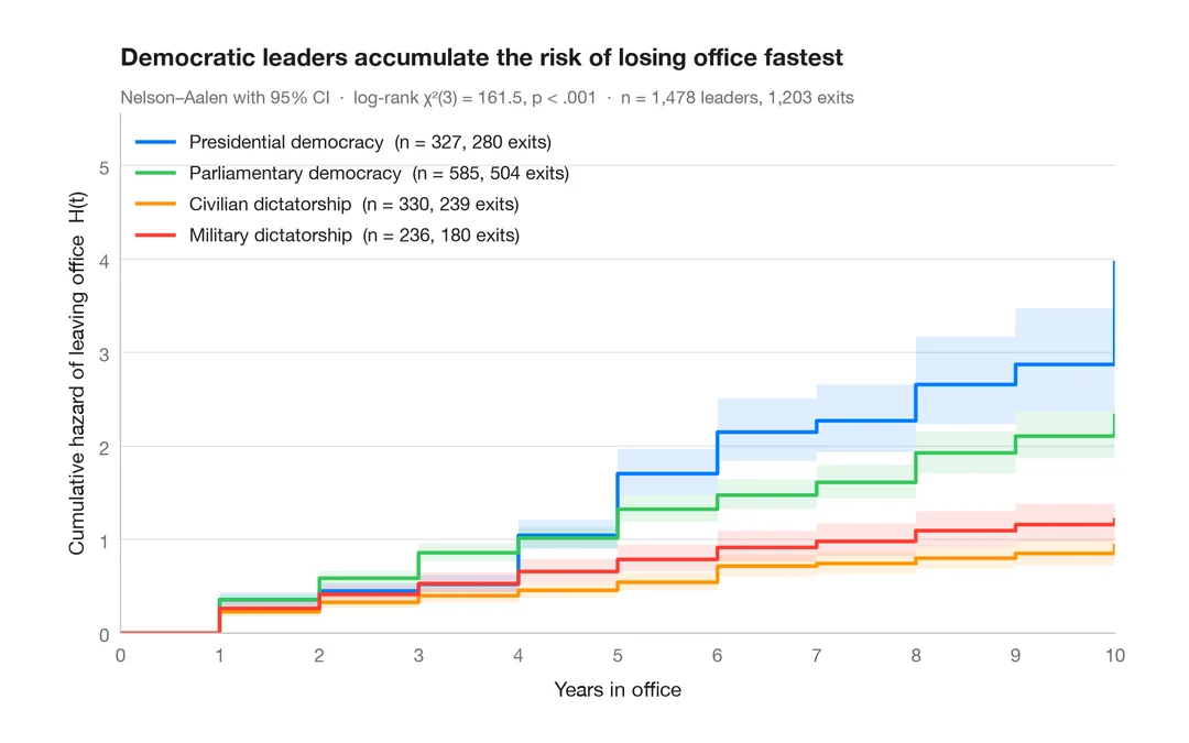
累積ハザード
4 つの政治体制について、退任の Nelson–Aalen 累積ハザードを 95% 信頼帯とともに示します。
survminer::ggsurvplot(fun = "cumhaz")