调整后的生存曲线
Cox 模型针对不同年龄预测的生存曲线,其他协变量固定在均值。
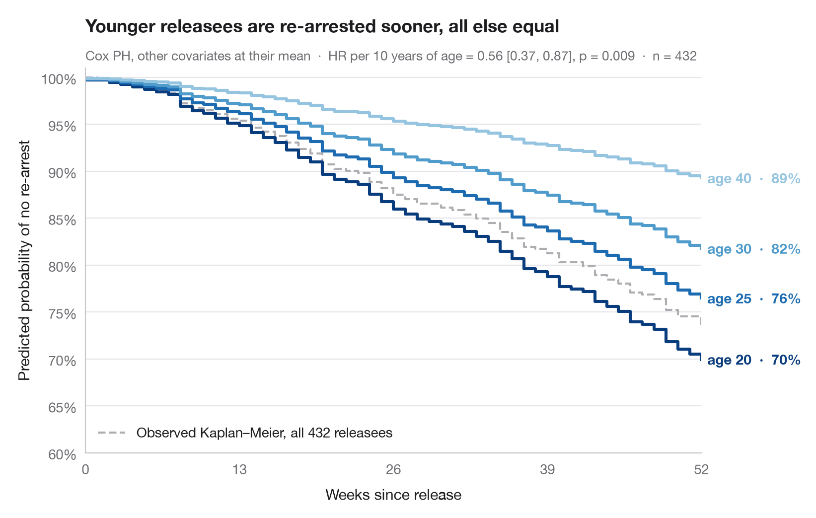
风险比难以直观感受,生存曲线则不然。这里使用拟合好的 Cox 比例风险模型,为仅在年龄上不同的假想个体预测完整的生存曲线,其他所有协变量都固定在样本均值。曲线之间的纵向差距,就是年龄效应换算成保持未被捕概率后的结果。
数据为 Rossi 再犯研究(lifelines.datasets.load_rossi)。模型用 lifelines.CoxPHFitter 基于全部七个协变量拟合,曲线来自 predict_survival_function();整个样本观测到的 Kaplan–Meier 曲线以灰色绘制作为参照。
代码及图中文字均为英文。
import matplotlib.pyplot as plt
import numpy as np
import pandas as pd
from lifelines import CoxPHFitter, KaplanMeierFitter
from lifelines.datasets import load_rossi

# Data: weeks to re-arrest after release from prison
df = load_rossi()
cph = CoxPHFitter().fit(df, duration_col="week", event_col="arrest")

# Hypothetical profiles: everything at the mean, age varies
ages = [20, 25, 30, 40]
profiles = pd.DataFrame([df.drop(columns=["week", "arrest"]).mean()] * len(ages))
profiles["age"] = ages
surv = cph.predict_survival_function(profiles, times=np.arange(0, 53))
colors = plt.cm.Blues(np.linspace(0.95, 0.4, len(ages)))

fig, ax = plt.subplots(figsize=(8, 5))

# Observed Kaplan–Meier curve of the whole sample, for reference
km = KaplanMeierFitter().fit(df.week, df.arrest)
ax.step(km.survival_function_.index, km.survival_function_.iloc[:, 0], where="post",
        color="#AEAEB2", lw=1.5, ls="--", label=f"Observed Kaplan–Meier, all {len(df)} releasees")
ax.legend(loc="lower left")

# Model-predicted curves, labelled at their end
for col, age, c in zip(surv.columns, ages, colors):
    s = surv[col]
    ax.step(s.index, s, where="post", color=c, lw=2.2)
    ax.text(52.5, s.iloc[-1], f"age {age}  ·  {s.iloc[-1]:.0%}", va="center",
            fontsize=10, color=c, fontweight="semibold")

hr10 = np.exp(10 * cph.params_["age"])
lo, hi = np.exp(10 * cph.confidence_intervals_.loc["age"])
p = cph.summary.loc["age", "p"]
ax.set(xlim=(0, 52), ylim=(0.6, 1.01), xticks=range(0, 53, 13),
       xlabel="Weeks since release", ylabel="Predicted probability of no re-arrest")
ax.yaxis.set_major_formatter(plt.matplotlib.ticker.PercentFormatter(1, decimals=0))
ax.set_title("Younger releasees are re-arrested sooner, all else equal", pad=26)
ax.text(0, 1.02, f"Cox PH, other covariates at their mean  ·  HR per 10 years of age = "
        f"{hr10:.2f} [{lo:.2f}, {hi:.2f}], p = {p:.3f}  ·  n = {len(df)}",
        transform=ax.transAxes, fontsize=9.5, color="#6E6E73")
plt.show()
图表使用了可选的 PyStatlas 样式:添加 plt.style.use("pystatlas.mplstyle") 即可完全还原其外观。
数据来源
- Rossi recidivism experiment (432 released prisoners). Rossi, P. H., Berk, R. A., & Lenihan, K. J. (1980). Money, Work, and Crime: Some Experimental Results. Academic Press. https://lifelines.readthedocs.io/en/latest/lifelines.datasets.html
Men released from Maryland state prisons in the 1970s, half randomly assigned to financial aid. Distributed with lifelines (lifelines.datasets.load_rossi).
这些示例用于说明统计方法。图表标题描述的是该图在这些特定数据中呈现的内容——这些数据往往样本较小、年代较早或并不完整——而不是作者对实质问题的立场。关于解释、背景和数据质量,请以此处引用的原始来源为准。
如何引用
PyStatlas 由 Thierry Warin 创建并维护。如果它对你的工作有所帮助,敬请引用。
Warin, T. (2026). Adjusted survival curves. In PyStatlas: A Python Gallery of Statistical Graphics for the Social Sciences. https://warint.github.io/pystatlas/survival/adjusted-survival/
@misc{warin2026statlas,
  author       = {Warin, Thierry},
  title        = {PyStatlas: A Python Gallery of Statistical Graphics for the Social Sciences},
  year         = {2026},
  howpublished = {\url{https://warint.github.io/pystatlas/}},
  note         = {Source code: https://github.com/warint/pystatlas}
}