Cox hazard ratios
Forest plot of a Cox proportional hazards model with HR, 95% CI and p-values.
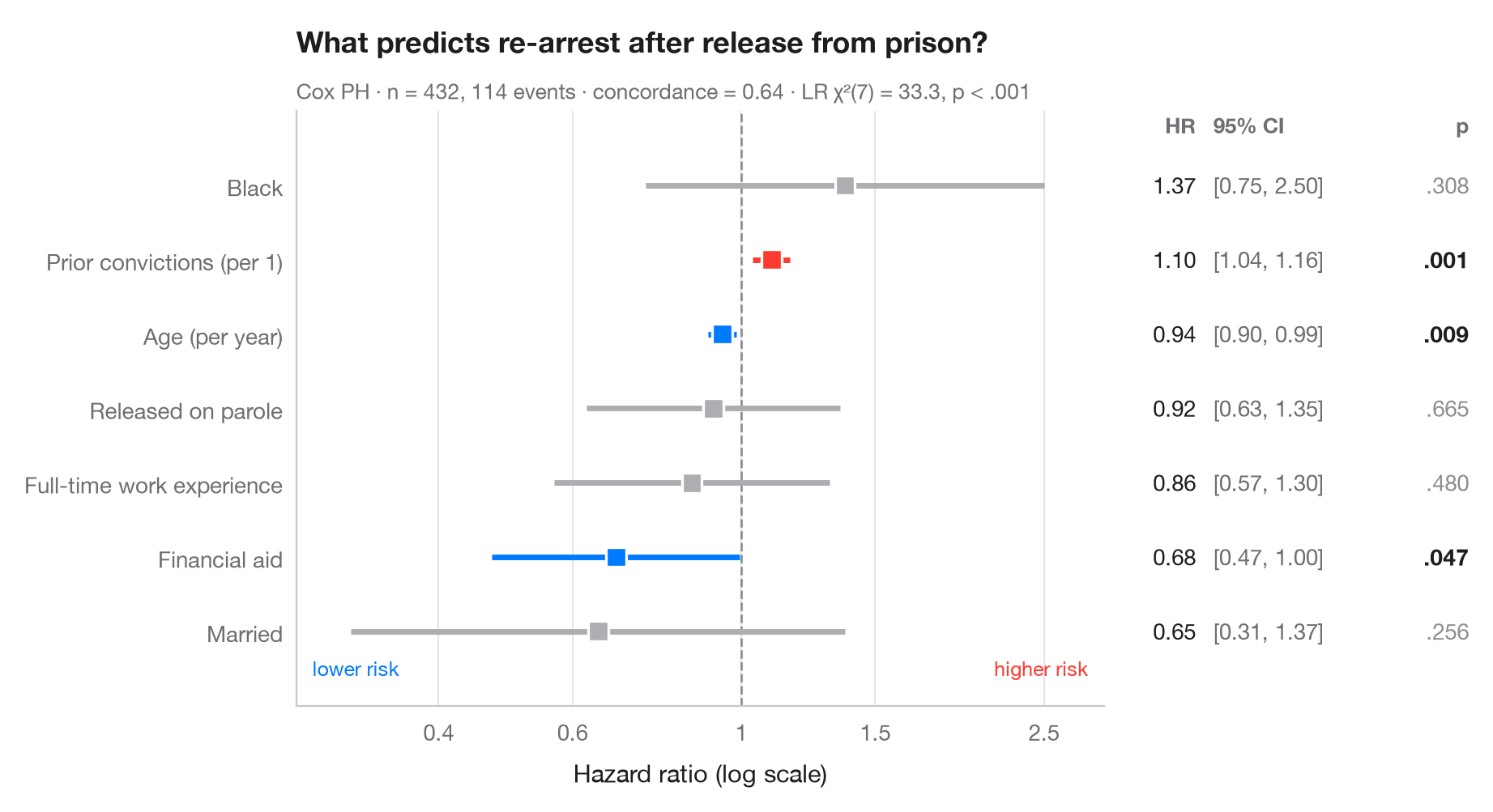
A Cox proportional hazards model estimates how each covariate multiplies the instantaneous risk of the event. Each row shows a hazard ratio (HR) with its 95% confidence interval on a log scale, so that halving and doubling the risk sit at equal distances from the reference line at HR = 1. The table on the right repeats the numbers, as in a published forest plot.
Data are the Rossi recidivism study (lifelines.datasets.load_rossi): 432
released prisoners followed for one year, the event being re-arrest. The model
is fitted with lifelines.CoxPHFitter; the subtitle reports the concordance
index and the likelihood-ratio test of the whole model.
import matplotlib.pyplot as plt
import numpy as np
from lifelines import CoxPHFitter
from lifelines.datasets import load_rossi

# Data: weeks to re-arrest after release from prison
df = load_rossi()
cph = CoxPHFitter().fit(df, duration_col="week", event_col="arrest")
lr = cph.log_likelihood_ratio_test()

# Tidy the summary: HR, 95% CI, p-value
labels = {"fin": "Financial aid", "age": "Age (per year)", "race": "Black",
          "wexp": "Full-time work experience", "mar": "Married",
          "paro": "Released on parole", "prio": "Prior convictions (per 1)"}
res = cph.summary.rename(columns={"exp(coef)": "hr", "exp(coef) lower 95%": "low",
                                  "exp(coef) upper 95%": "high"})
res = res.sort_values("hr")
y = np.arange(len(res))
colors = np.where(res.p < 0.05, np.where(res.hr > 1, "#FF3B30", "#007AFF"), "#AEAEB2")

fig, (ax, tab) = plt.subplots(1, 2, figsize=(9, 4.8), sharey=True,
                              gridspec_kw=dict(width_ratios=[3, 1.3]))

# Forest: CI whiskers and point estimates on a log axis
ax.axvline(1, color="#8E8E93", lw=1, ls="--", zorder=1)
ax.hlines(y, res.low, res.high, color=colors, lw=2.5, zorder=2)
ax.scatter(res.hr, y, s=80, marker="s", color=colors, edgecolor="white", lw=1.2, zorder=3)
ax.set_xscale("log")
ax.set_xticks([0.4, 0.6, 1, 1.5, 2.5], ["0.4", "0.6", "1", "1.5", "2.5"])
ax.minorticks_off()
ax.set_xlim(0.26, 3)
ax.set_yticks(y, [labels[t] for t in res.index])
ax.grid(axis="x"); ax.grid(axis="y", visible=False)
ax.set_xlabel("Hazard ratio (log scale)")
ax.text(0.98, -0.6, "higher risk", ha="right", color="#FF3B30", fontsize=9,
        transform=ax.get_yaxis_transform())
ax.text(0.02, -0.6, "lower risk", ha="left", color="#007AFF", fontsize=9,
        transform=ax.get_yaxis_transform())

# Table: HR [95% CI] and p-value
for yi, (_, r) in zip(y, res.iterrows()):
    p = "< .001" if r.p < 0.001 else f"{r.p:.3f}".lstrip("0")
    tab.text(0.22, yi, f"{r.hr:.2f}", va="center", ha="right", fontsize=10, color="#1D1D1F")
    tab.text(0.27, yi, f"[{r.low:.2f}, {r.high:.2f}]", va="center", fontsize=10, color="#6E6E73")
    tab.text(1, yi, p, va="center", ha="right", fontsize=10,
             color="#1D1D1F" if r.p < 0.05 else "#8E8E93",
             fontweight="semibold" if r.p < 0.05 else "normal")
tab.text(0.22, len(res) - 0.3, "HR", ha="right", fontsize=9.5, color="#6E6E73", fontweight="semibold")
tab.text(0.27, len(res) - 0.3, "95% CI", fontsize=9.5, color="#6E6E73", fontweight="semibold")
tab.text(1, len(res) - 0.3, "p", ha="right", fontsize=9.5, color="#6E6E73", fontweight="semibold")
tab.set(xlim=(0, 1), ylim=(-1, len(res)))
tab.axis("off")

ax.set_title("What predicts re-arrest after release from prison?", pad=26)
ax.text(0, 1.02, f"Cox PH · n = {len(df)}, {df.arrest.sum()} events · concordance = "
        f"{cph.concordance_index_:.2f} · LR χ²({lr.degrees_freedom:.0f}) = {lr.test_statistic:.1f}, "
        f"p < .001", transform=ax.transAxes, fontsize=9.5, color="#6E6E73")
plt.show()
Figures use the optional PyStatlas style: add plt.style.use("pystatlas.mplstyle") to match the look exactly.
Data source
- Rossi recidivism experiment (432 released prisoners). Rossi, P. H., Berk, R. A., & Lenihan, K. J. (1980). Money, Work, and Crime: Some Experimental Results. Academic Press. https://lifelines.readthedocs.io/en/latest/lifelines.datasets.html
Men released from Maryland state prisons in the 1970s, half randomly assigned to financial aid. Distributed with lifelines (lifelines.datasets.load_rossi).
The examples illustrate statistical methods. Their titles describe what each figure shows in these particular data — often a small, dated or partial sample — not the author's position on the substantive question. For interpretation, context and data quality, rely on the original sources cited here.
How to cite
PyStatlas is created and maintained by Thierry Warin. If it helped your work, please cite it.
Warin, T. (2026). Cox hazard ratios. In PyStatlas: A Python Gallery of Statistical Graphics for the Social Sciences. https://warint.github.io/pystatlas/survival/cox-hazard-ratios/
@misc{warin2026statlas,
  author       = {Warin, Thierry},
  title        = {PyStatlas: A Python Gallery of Statistical Graphics for the Social Sciences},
  year         = {2026},
  howpublished = {\url{https://warint.github.io/pystatlas/}},
  note         = {Source code: https://github.com/warint/pystatlas}
}More in Survival analysis
Kaplan–Meier curves
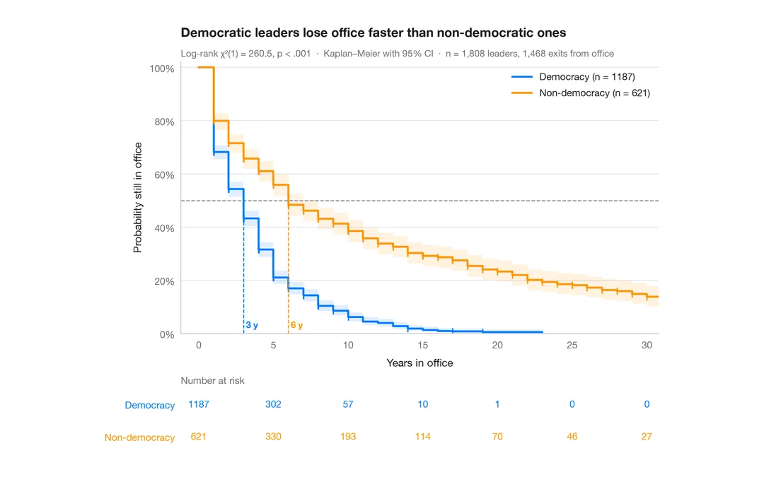
How long political leaders stay in office, democracies vs non-democracies — survival curves with confidence bands, censoring marks, log-rank test and risk table.
survminer::ggsurvplot(risk.table = TRUE)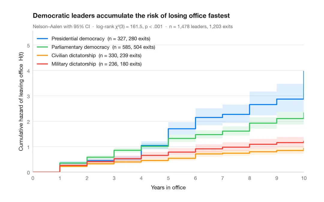
Cumulative hazard
Nelson–Aalen cumulative hazard of leaving office, with 95% bands, for four political regimes.
survminer::ggsurvplot(fun = "cumhaz")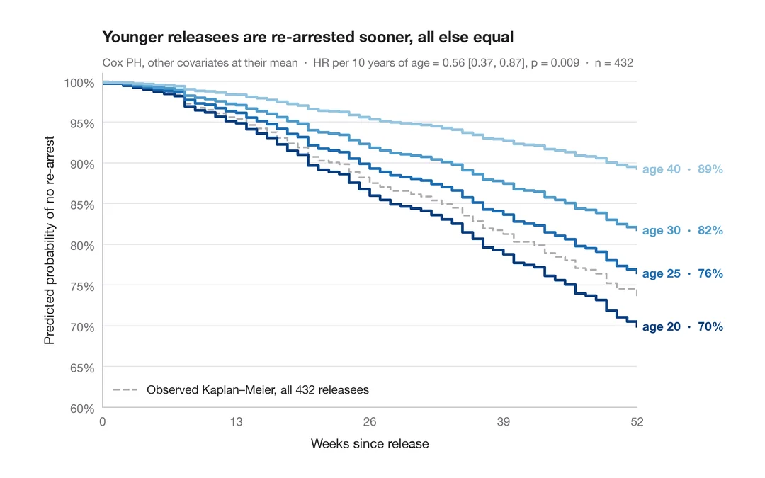
Adjusted survival curves
Cox model–predicted survival for several ages, other covariates held at their mean.
survminer::ggadjustedcurves()