Cross-validated model comparison
Fold-by-fold R² of six models predicting California school districts' maths results, with means and corrected 95% intervals.
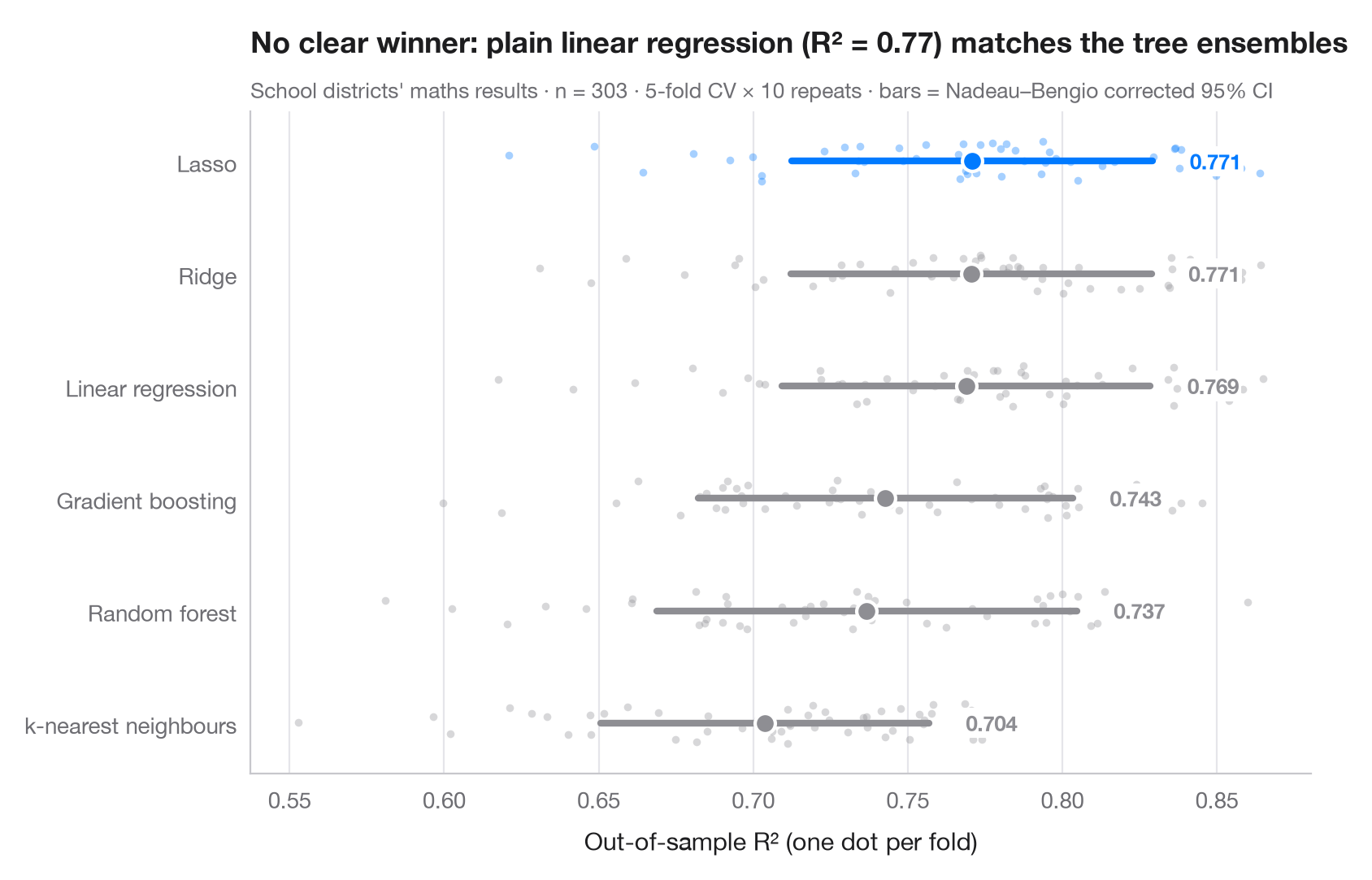
"Model B scores 0.47, model A 0.46" says nothing until we know how much the score moves from one split to the next. Here every model is evaluated on the same 10 × 5 repeated folds; each dot is one fold, the large marker is the mean and the bar its 95% interval. Fold scores are not independent — the training sets overlap — so the interval uses the Nadeau–Bengio corrected variance rather than the naive standard error, which would be far too narrow.
Data are the 303 California school districts of the 1998 STAR test bundled
with statsmodels (sm.datasets.star98): the outcome is the share of
students scoring above the national median in maths, predicted from ten
district characteristics (share of low-income students, ethnic composition,
teacher experience and salary, spending per pupil, pupils per teacher,
college-prep enrolment, year-round schools). The score is the out-of-sample
R². Scores come from cross_val_score with RepeatedKFold; the linear models
are standardised in a Pipeline. Here plain linear regression does as well
as the tree ensembles: flexibility buys nothing when the relationship is close
to additive.
import matplotlib.pyplot as plt
import numpy as np
from scipy import stats
import statsmodels.api as sm
from sklearn.ensemble import GradientBoostingRegressor, RandomForestRegressor
from sklearn.linear_model import LassoCV, LinearRegression, RidgeCV
from sklearn.model_selection import RepeatedKFold, cross_val_score
from sklearn.neighbors import KNeighborsRegressor
from sklearn.pipeline import make_pipeline
from sklearn.preprocessing import StandardScaler

# Data: 303 California school districts; outcome = % of students above the national median in maths
d = sm.datasets.star98.load_pandas().data
y = 100 * d["NABOVE"] / (d["NABOVE"] + d["NBELOW"])
names = {"LOWINC": "% low-income students", "PERASIAN": "% Asian students", "PERBLACK": "% Black students",
         "PERHISP": "% Hispanic students", "AVYRSEXP": "Teacher experience (years)",
         "AVSALK": "Teacher salary ($000)", "PERSPENK": "Spending per pupil ($000)",
         "PTRATIO": "Pupils per teacher", "PCTAF": "% in college-prep courses",
         "PCTYRRND": "% year-round schools"}
X = d[list(names)]
k, reps = 5, 10
cv = RepeatedKFold(n_splits=k, n_repeats=reps, random_state=0)
models = {
    "Linear regression": make_pipeline(StandardScaler(), LinearRegression()),
    "Ridge": make_pipeline(StandardScaler(), RidgeCV(alphas=np.logspace(-3, 3, 25))),
    "Lasso": make_pipeline(StandardScaler(), LassoCV(random_state=0)),
    "Random forest": RandomForestRegressor(n_estimators=300, min_samples_leaf=5, random_state=0),
    "Gradient boosting": GradientBoostingRegressor(learning_rate=0.05, max_depth=2, random_state=0),
    "k-nearest neighbours": make_pipeline(StandardScaler(), KNeighborsRegressor(n_neighbors=15)),
}
scores = {name: cross_val_score(m, X, y, cv=cv, scoring="r2", n_jobs=-1) for name, m in models.items()}

# Nadeau–Bengio corrected 95% interval for a mean of k-fold scores
def corrected_ci(s):
    J = len(s)
    se = np.sqrt((1 / J + (1 / k) / (1 - 1 / k)) * s.var(ddof=1))
    t = stats.t.ppf(0.975, J - 1)
    return s.mean() - t * se, s.mean() + t * se

order = sorted(scores, key=lambda n: scores[n].mean())
best = order[-1]
fig, ax = plt.subplots(figsize=(8, 5.2))
rng = np.random.default_rng(3)
for i, name in enumerate(order):
    s = scores[name]
    c = "#007AFF" if name == best else "#8E8E93"
    ax.scatter(s, i + rng.uniform(-0.18, 0.18, len(s)), s=12, color=c, alpha=0.35, lw=0)
    lo, hi = corrected_ci(s)
    ax.plot([lo, hi], [i, i], color=c, lw=3, solid_capstyle="round")
    ax.scatter(s.mean(), i, s=80, color=c, edgecolor="white", lw=1.5, zorder=4)
    ax.text(hi + 0.012, i, f"{s.mean():.3f}", va="center", fontsize=9.5, color=c, fontweight="semibold",
            bbox=dict(fc="white", ec="none", pad=1), zorder=5)
ax.set_yticks(range(len(order)), order)
ax.set_xlabel("Out-of-sample R² (one dot per fold)")
ax.grid(axis="x"); ax.grid(axis="y", visible=False)
lin = scores["Linear regression"].mean()
ax.set_title(f"No clear winner: plain linear regression (R² = {lin:.2f}) matches the tree ensembles", pad=26)
ax.text(0, 1.02, f"School districts' maths results · n = {len(y)} · {k}-fold CV × {reps} repeats · "
        "bars = Nadeau–Bengio corrected 95% CI", transform=ax.transAxes, fontsize=9.5, color="#6E6E73")
plt.show()
Figures use the optional PyStatlas style: add plt.style.use("pystatlas.mplstyle") to match the look exactly.
Data source
- California STAR test results, 1998 (303 school districts). Gill, J. (2001). Generalized Linear Models: A Unified Approach (Quantitative Applications in the Social Sciences, No. 134). Sage. https://www.statsmodels.org/stable/datasets/generated/star98.html
Original data from the California Department of Education's Standardized Testing and Reporting (STAR) program, 1998. Subset distributed with statsmodels (sm.datasets.star98) with the author's permission.
The examples illustrate statistical methods. Their titles describe what each figure shows in these particular data — often a small, dated or partial sample — not the author's position on the substantive question. For interpretation, context and data quality, rely on the original sources cited here.
How to cite
PyStatlas is created and maintained by Thierry Warin. If it helped your work, please cite it.
Warin, T. (2026). Cross-validated model comparison. In PyStatlas: A Python Gallery of Statistical Graphics for the Social Sciences. https://warint.github.io/pystatlas/machine-learning/model-comparison/
@misc{warin2026statlas,
  author       = {Warin, Thierry},
  title        = {PyStatlas: A Python Gallery of Statistical Graphics for the Social Sciences},
  year         = {2026},
  howpublished = {\url{https://warint.github.io/pystatlas/}},
  note         = {Source code: https://github.com/warint/pystatlas}
}More in Machine learning
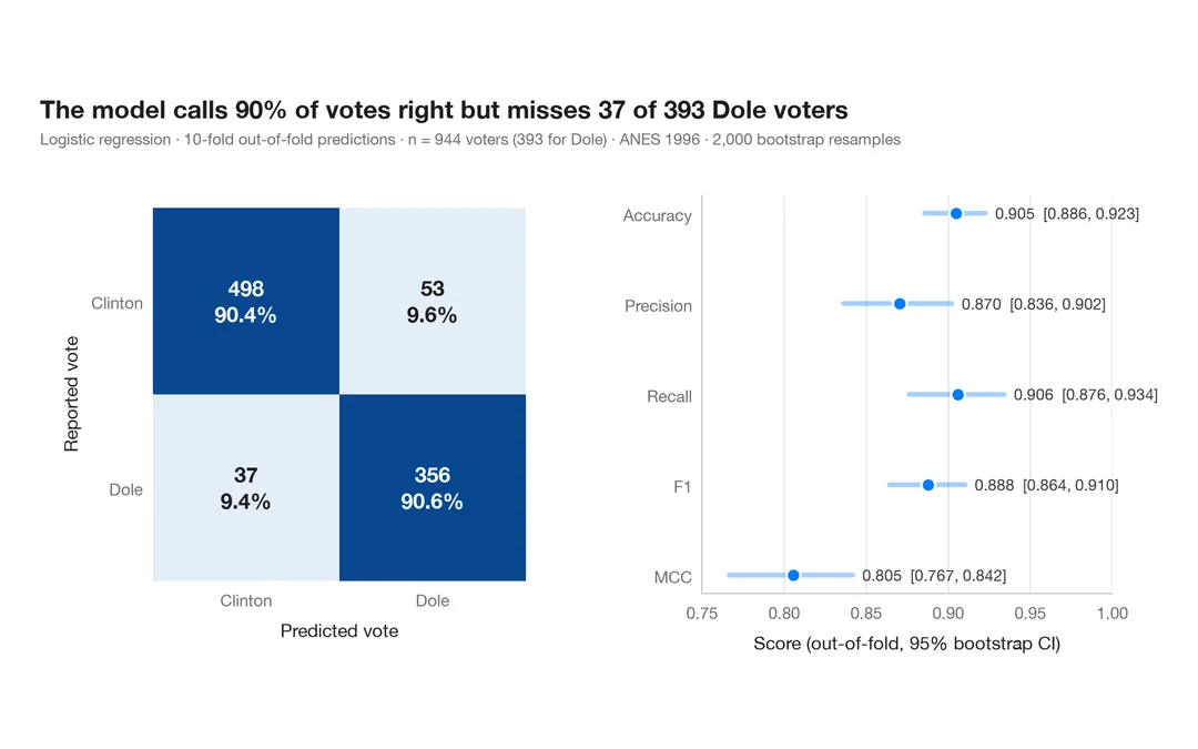
Confusion matrix with metrics
How well a logistic regression predicts who voted Dole in 1996 — out-of-fold confusion matrix with counts and row shares, and bootstrap intervals for the headline metrics.
yardstick::conf_mat() + autoplot()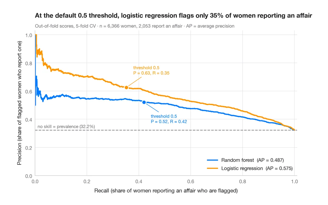
Precision–recall curves
Out-of-fold precision–recall curves for two classifiers predicting which married women report an affair, with average precision and the no-skill baseline.
yardstick::pr_curve() + autoplot()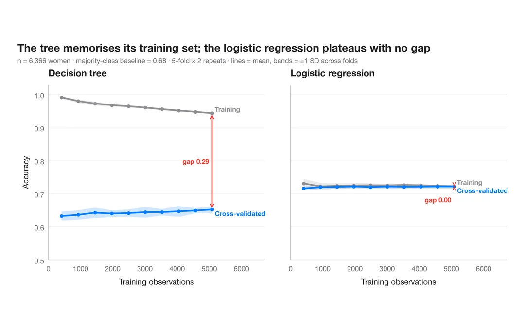
Learning curve
Training and cross-validated accuracy as the training set grows, for two models predicting which married women report an affair.
caret::learning_curve_dat() + ggplot()