Learning curve
Training and cross-validated accuracy as the training set grows, for two models predicting which married women report an affair.
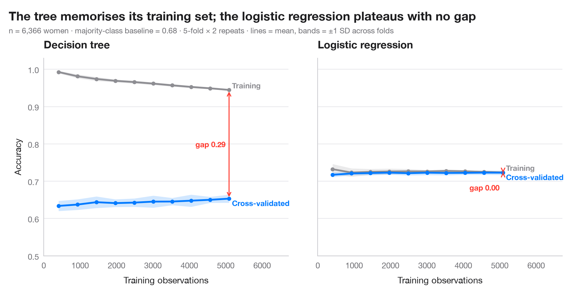
A learning curve answers two questions before anyone collects more data: is the model overfitting (a wide gap between the training score and the cross-validated score) or underfitting (both scores low and close), and would more observations still help (is the validation curve still rising)? Lines are means over the folds of a repeated cross-validation; bands are ±1 standard deviation, so the width shows how much the estimate would move with another split.
Two models are compared on the same task: a deep decision tree, which
memorises its training set, and a standardised logistic regression. Data are
the 6,366 married women of the 1974 Redbook magazine survey analysed by Fair
(1978), bundled with statsmodels (sm.datasets.fair); the outcome is
whether a woman reports any extramarital affair (about one in three), predicted
from her rating of the marriage, age, years married, children, religiousness,
education and occupations. The curves come from
sklearn.model_selection.learning_curve with a 5 × 2 repeated stratified
split. The verdict is sobering: the tree's cross-validated accuracy stays
below the majority-class baseline, while the logistic regression's two curves
are flat and joined — more respondents would not help; better predictors
would.
import matplotlib.pyplot as plt
import numpy as np
import statsmodels.api as sm
from sklearn.linear_model import LogisticRegression
from sklearn.model_selection import RepeatedStratifiedKFold, learning_curve
from sklearn.pipeline import make_pipeline
from sklearn.preprocessing import StandardScaler
from sklearn.tree import DecisionTreeClassifier

# Data: 6,366 married women (1974 survey); 1 = reports any extramarital affair
d = sm.datasets.fair.load_pandas().data
X = d.drop(columns="affairs")
y = (d["affairs"] > 0).astype(int)
cv = RepeatedStratifiedKFold(n_splits=5, n_repeats=2, random_state=0)
sizes = np.linspace(0.08, 1.0, 10)
models = {"Decision tree": DecisionTreeClassifier(random_state=0),
          "Logistic regression": make_pipeline(StandardScaler(), LogisticRegression(max_iter=1000))}

plt.rcParams["figure.constrained_layout.use"] = False   # manual margins leave room for the subtitle
fig, axes = plt.subplots(1, 2, figsize=(10, 5), sharey=True)
fig.subplots_adjust(left=0.08, right=0.97, top=0.80, bottom=0.12, wspace=0.12)
for ax, (name, model) in zip(axes, models.items()):
    n, train, valid = learning_curve(model, X, y, cv=cv, train_sizes=sizes, n_jobs=-1,
                                    shuffle=True, random_state=0)   # rows are sorted by outcome
    for scores, c, lab in [(train, "#8E8E93", "Training"), (valid, "#007AFF", "Cross-validated")]:
        m, s = scores.mean(axis=1), scores.std(axis=1)
        ax.fill_between(n, m - s, m + s, color=c, alpha=0.18, lw=0)
        ax.plot(n, m, color=c, lw=2.2, marker="o", ms=4)
        dy = 0.012 if lab == "Training" else -0.012
        ax.text(n[-1] + 80, m[-1] + dy, lab, va="center", fontsize=9.5, color=c, fontweight="semibold")
    gap = train.mean(axis=1)[-1] - valid.mean(axis=1)[-1]
    ax.annotate("", xy=(n[-1], valid.mean(axis=1)[-1]), xytext=(n[-1], train.mean(axis=1)[-1]),
                arrowprops=dict(arrowstyle="<->", color="#FF3B30", lw=1.2))
    ax.text(n[-1] - 100, valid.mean(axis=1)[-1] + (gap / 2 if gap > 0.05 else -0.04), f"gap {gap:.2f}",
            ha="right", va="center", fontsize=9.5, color="#FF3B30", fontweight="semibold")
    ax.set_title(name)
    ax.set_xlabel("Training observations")
    ax.set_xlim(0, n[-1] * 1.32)
axes[0].set_ylabel("Accuracy")
axes[0].set_ylim(0.5, 1.03)

fig.suptitle("The tree memorises its training set; the logistic regression plateaus with no gap",
             x=0.02, y=0.97, ha="left")
fig.text(0.02, 0.885, f"n = {len(y):,} women · majority-class baseline = {1 - y.mean():.2f} · "
         "5-fold × 2 repeats · lines = mean, bands = ±1 SD across folds",
         fontsize=9.5, color="#6E6E73")
plt.show()
Figures use the optional PyStatlas style: add plt.style.use("pystatlas.mplstyle") to match the look exactly.
Data source
- Redbook survey of married women, 1974 (Fair's affairs data). Fair, R. C. (1978). A theory of extramarital affairs. Journal of Political Economy, 86(1), 45–61. https://doi.org/10.1086/260646
Data from the 1974 Redbook magazine survey; distributed with statsmodels (sm.datasets.fair) with the author's permission.
The examples illustrate statistical methods. Their titles describe what each figure shows in these particular data — often a small, dated or partial sample — not the author's position on the substantive question. For interpretation, context and data quality, rely on the original sources cited here.
How to cite
PyStatlas is created and maintained by Thierry Warin. If it helped your work, please cite it.
Warin, T. (2026). Learning curve. In PyStatlas: A Python Gallery of Statistical Graphics for the Social Sciences. https://warint.github.io/pystatlas/machine-learning/learning-curve/
@misc{warin2026statlas,
  author       = {Warin, Thierry},
  title        = {PyStatlas: A Python Gallery of Statistical Graphics for the Social Sciences},
  year         = {2026},
  howpublished = {\url{https://warint.github.io/pystatlas/}},
  note         = {Source code: https://github.com/warint/pystatlas}
}More in Machine learning
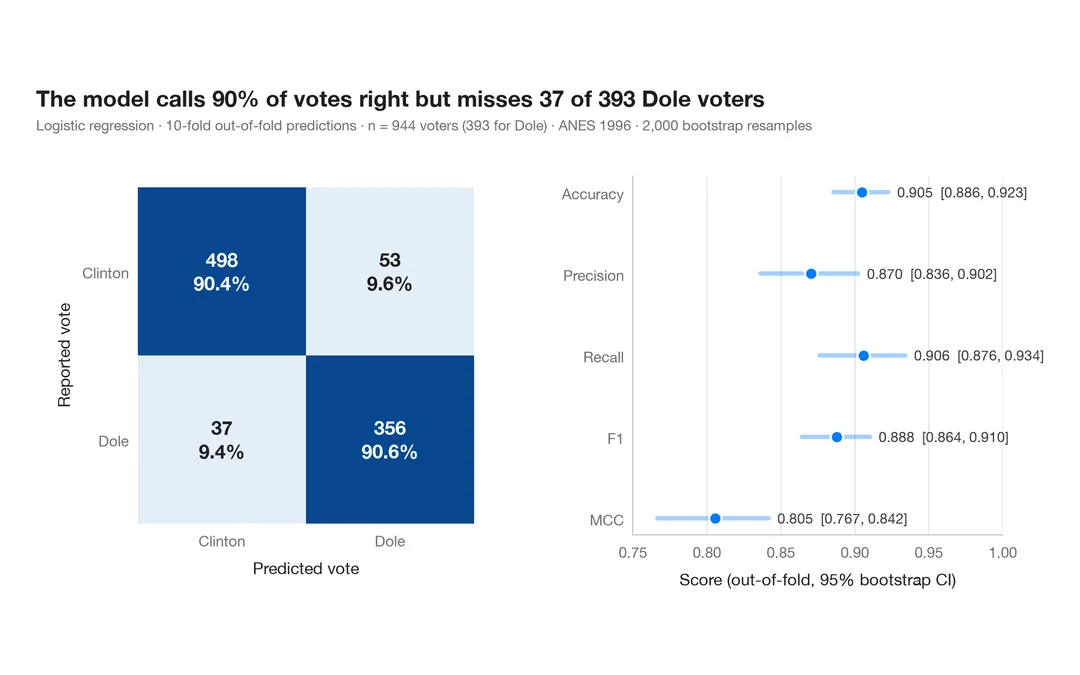
Confusion matrix with metrics
How well a logistic regression predicts who voted Dole in 1996 — out-of-fold confusion matrix with counts and row shares, and bootstrap intervals for the headline metrics.
yardstick::conf_mat() + autoplot()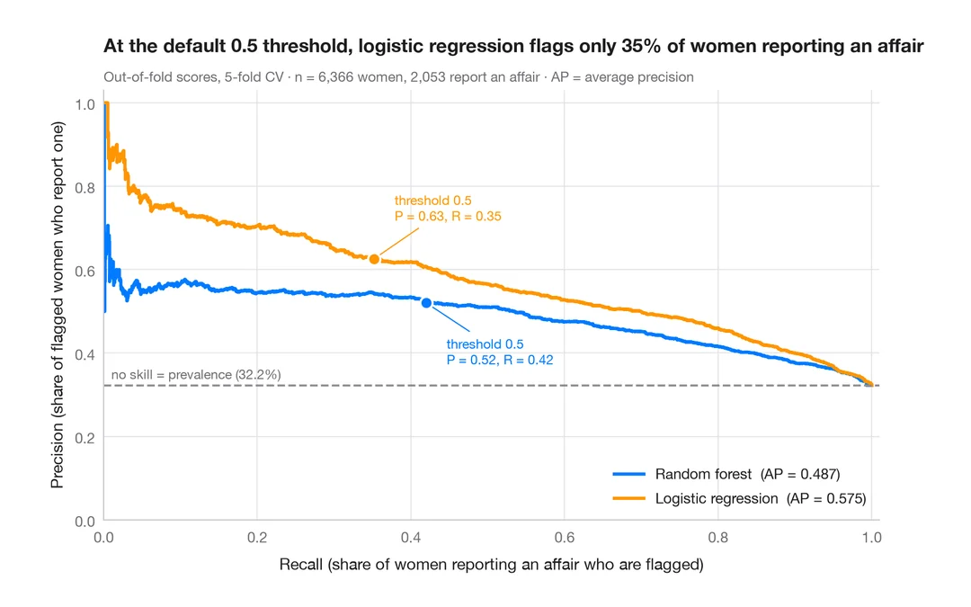
Precision–recall curves
Out-of-fold precision–recall curves for two classifiers predicting which married women report an affair, with average precision and the no-skill baseline.
yardstick::pr_curve() + autoplot()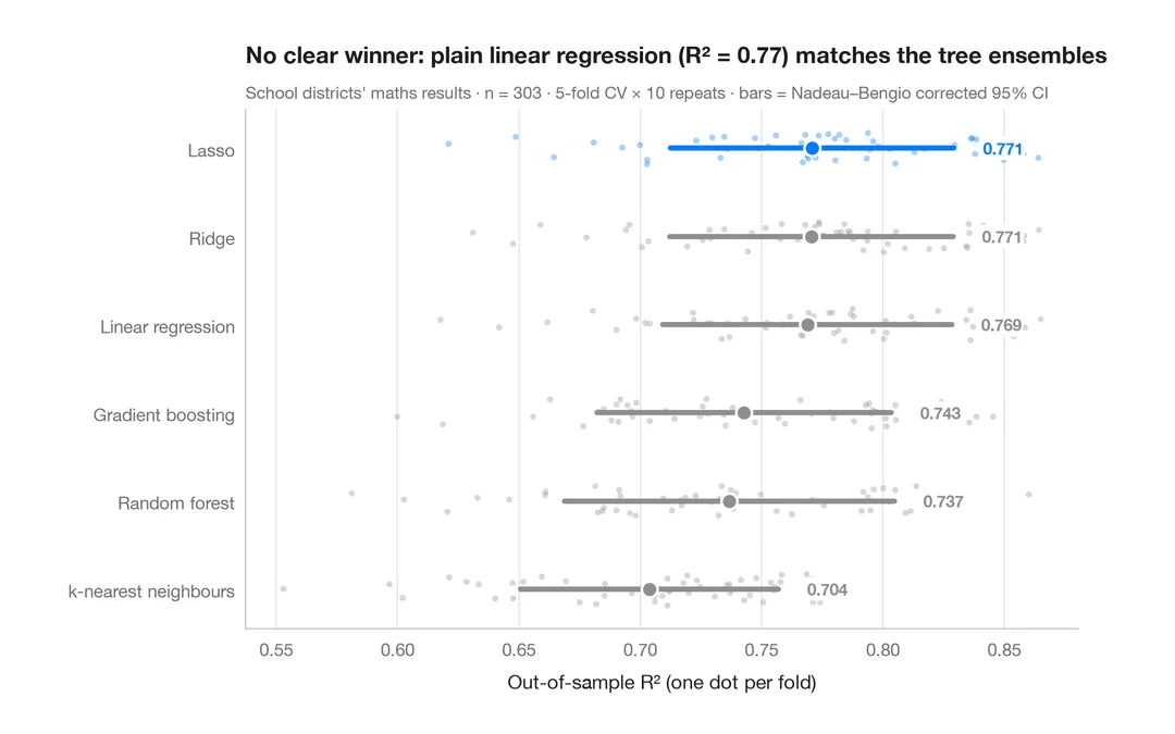
Cross-validated model comparison
Fold-by-fold R² of six models predicting California school districts' maths results, with means and corrected 95% intervals.
caret::resamples() + bwplot() / tune::autoplot()