Learning curve — PyStatlas: A Python Gallery of Statistical Graphics for the Social Sciences

Warin, Thierry

学習曲線

既婚女性のうち誰が婚外関係を申告するかを予測する 2 つのモデルについて、訓練データを増やしたときの訓練正解率と交差検証正解率を示します。

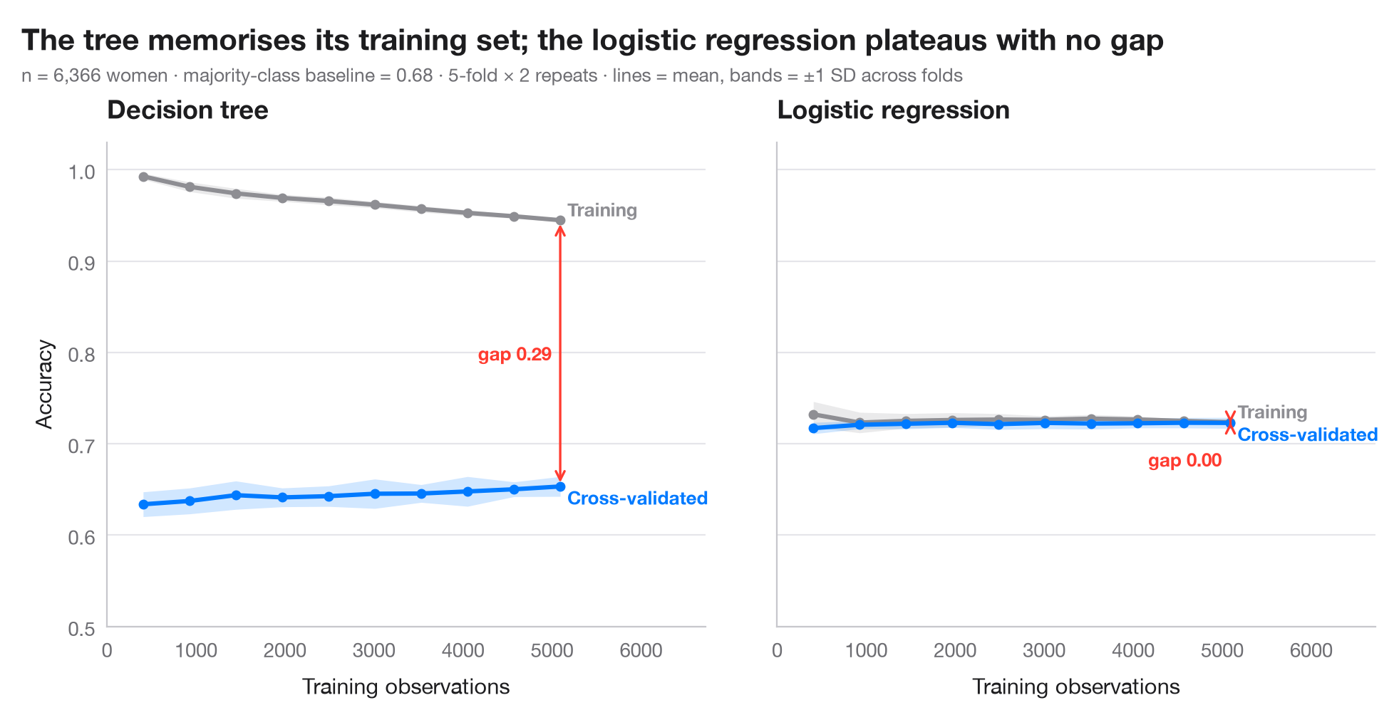
学習曲線は、データを追加で集める前に 2 つの問いに答えます。モデルは 過学習 しているか（訓練スコアと交差検証スコアの差が大きい）、それとも 学習不足 か（どちらのスコアも低く近い）。そして、観測値を増やせばまだ改善するか（検証曲線がまだ上がっているか）。線は反復交差検証の各分割の平均、帯は ±1 標準偏差で、その幅は別の分割で推定値がどれだけ動くかを示します。

同じ課題で 2 つのモデルを比べます。訓練データを丸暗記する深い決定木と、標準化したロジスティック回帰です。データは、Fair（1978）が分析した 1974 年の Redbook 誌調査の既婚女性 6,366 人で、statsmodels に付属しています（sm.datasets.fair）。目的変数は婚外関係を申告したかどうか（約 3 人に 1 人）で、結婚生活の評価、年齢、結婚年数、子ども、信仰の篤さ、学歴、職業から予測します。曲線は sklearn.model_selection.learning_curve に 5 × 2 の反復層化分割を用いて求めています。結論は厳しいものです。決定木の交差検証正解率は多数派クラスのベースラインを下回ったままで、ロジスティック回帰の 2 本の曲線は平らで重なっています。回答者を増やしても役に立たず、役に立つのはより良い予測変数です。

コードおよび図中のテキストは英語です。

learning-curve.py · 47 行

ダウンロード GitHub

import matplotlib.pyplot as plt
import numpy as np
import statsmodels.api as sm
from sklearn.linear_model import LogisticRegression
from sklearn.model_selection import RepeatedStratifiedKFold, learning_curve
from sklearn.pipeline import make_pipeline
from sklearn.preprocessing import StandardScaler
from sklearn.tree import DecisionTreeClassifier

# Data: 6,366 married women (1974 survey); 1 = reports any extramarital affair
d = sm.datasets.fair.load_pandas().data
X = d.drop(columns="affairs")
y = (d["affairs"] > 0).astype(int)
cv = RepeatedStratifiedKFold(n_splits=5, n_repeats=2, random_state=0)
sizes = np.linspace(0.08, 1.0, 10)
models = {"Decision tree": DecisionTreeClassifier(random_state=0),
          "Logistic regression": make_pipeline(StandardScaler(), LogisticRegression(max_iter=1000))}

plt.rcParams["figure.constrained_layout.use"] = False   # manual margins leave room for the subtitle
fig, axes = plt.subplots(1, 2, figsize=(10, 5), sharey=True)
fig.subplots_adjust(left=0.08, right=0.97, top=0.80, bottom=0.12, wspace=0.12)
for ax, (name, model) in zip(axes, models.items()):
    n, train, valid = learning_curve(model, X, y, cv=cv, train_sizes=sizes, n_jobs=-1,
                                    shuffle=True, random_state=0)   # rows are sorted by outcome
    for scores, c, lab in [(train, "#8E8E93", "Training"), (valid, "#007AFF", "Cross-validated")]:
        m, s = scores.mean(axis=1), scores.std(axis=1)
        ax.fill_between(n, m - s, m + s, color=c, alpha=0.18, lw=0)
        ax.plot(n, m, color=c, lw=2.2, marker="o", ms=4)
        dy = 0.012 if lab == "Training" else -0.012
        ax.text(n[-1] + 80, m[-1] + dy, lab, va="center", fontsize=9.5, color=c, fontweight="semibold")
    gap = train.mean(axis=1)[-1] - valid.mean(axis=1)[-1]
    ax.annotate("", xy=(n[-1], valid.mean(axis=1)[-1]), xytext=(n[-1], train.mean(axis=1)[-1]),
                arrowprops=dict(arrowstyle="<->", color="#FF3B30", lw=1.2))
    ax.text(n[-1] - 100, valid.mean(axis=1)[-1] + (gap / 2 if gap > 0.05 else -0.04), f"gap {gap:.2f}",
            ha="right", va="center", fontsize=9.5, color="#FF3B30", fontweight="semibold")
    ax.set_title(name)
    ax.set_xlabel("Training observations")
    ax.set_xlim(0, n[-1] * 1.32)
axes[0].set_ylabel("Accuracy")
axes[0].set_ylim(0.5, 1.03)

fig.suptitle("The tree memorises its training set; the logistic regression plateaus with no gap",
             x=0.02, y=0.97, ha="left")
fig.text(0.02, 0.885, f"n = {len(y):,} women · majority-class baseline = {1 - y.mean():.2f} · "
         "5-fold × 2 repeats · lines = mean, bands = ±1 SD across folds",
         fontsize=9.5, color="#6E6E73")
plt.show()

図にはオプションの PyStatlas スタイルを使用しています。同じ見た目にするには plt.style.use("pystatlas.mplstyle") を追加してください。

データの出典

Redbook survey of married women, 1974 (Fair's affairs data). Fair, R. C. (1978). A theory of extramarital affairs. Journal of Political Economy, 86(1), 45–61. https://doi.org/10.1086/260646
Data from the 1974 Redbook magazine survey; distributed with statsmodels (sm.datasets.fair) with the author's permission.

これらの例は統計手法を説明するためのものです。図のタイトルは、この特定のデータ（多くは小規模で、古く、部分的な標本）で図が示す内容を述べたものであり、実質的な問いに対する著者の立場ではありません。解釈、背景、データの質については、ここに挙げた元の出典を参照してください。

引用方法

PyStatlas は Thierry Warin が作成・運営しています。研究や業務に役立った場合は、ぜひ引用してください。

Warin, T. (2026). Learning curve. In PyStatlas: A Python Gallery of Statistical Graphics for the Social Sciences. https://warint.github.io/pystatlas/machine-learning/learning-curve/

@misc{warin2026statlas,
  author       = {Warin, Thierry},
  title        = {PyStatlas: A Python Gallery of Statistical Graphics for the Social Sciences},
  year         = {2026},
  howpublished = {\url{https://warint.github.io/pystatlas/}},
  note         = {Source code: https://github.com/warint/pystatlas}
}

機械学習のその他のグラフ

機械学習

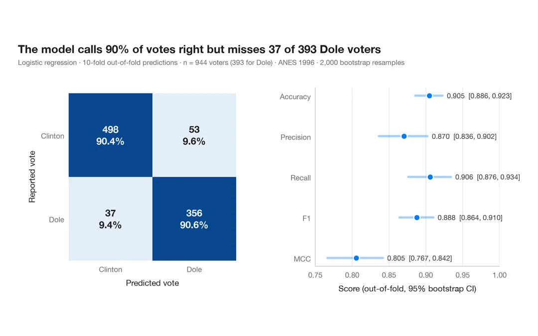
指標付き混同行列

1996 年にドールに投票した人をロジスティック回帰がどれだけ当てられるか。件数と行ごとの割合を示す交差検証の混同行列に、主要指標のブートストラップ区間を添えます。

yardstick::conf_mat() + autoplot()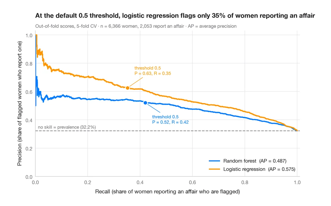

機械学習

適合率–再現率曲線

既婚女性のうち誰が婚外関係を申告するかを予測する 2 つの分類器の、交差検証による適合率–再現率曲線と、平均適合率、無技能のベースライン。

yardstick::pr_curve() + autoplot()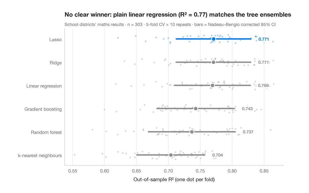

機械学習

交差検証によるモデル比較

カリフォルニア州の学区の数学の成績を予測する 6 つのモデルの分割ごとの R² を、平均値と補正済み 95% 区間とともに示します。

caret::resamples() + bwplot() / tune::autoplot()