適合率–再現率曲線
既婚女性のうち誰が婚外関係を申告するかを予測する 2 つの分類器の、交差検証による適合率–再現率曲線と、平均適合率、無技能のベースライン。
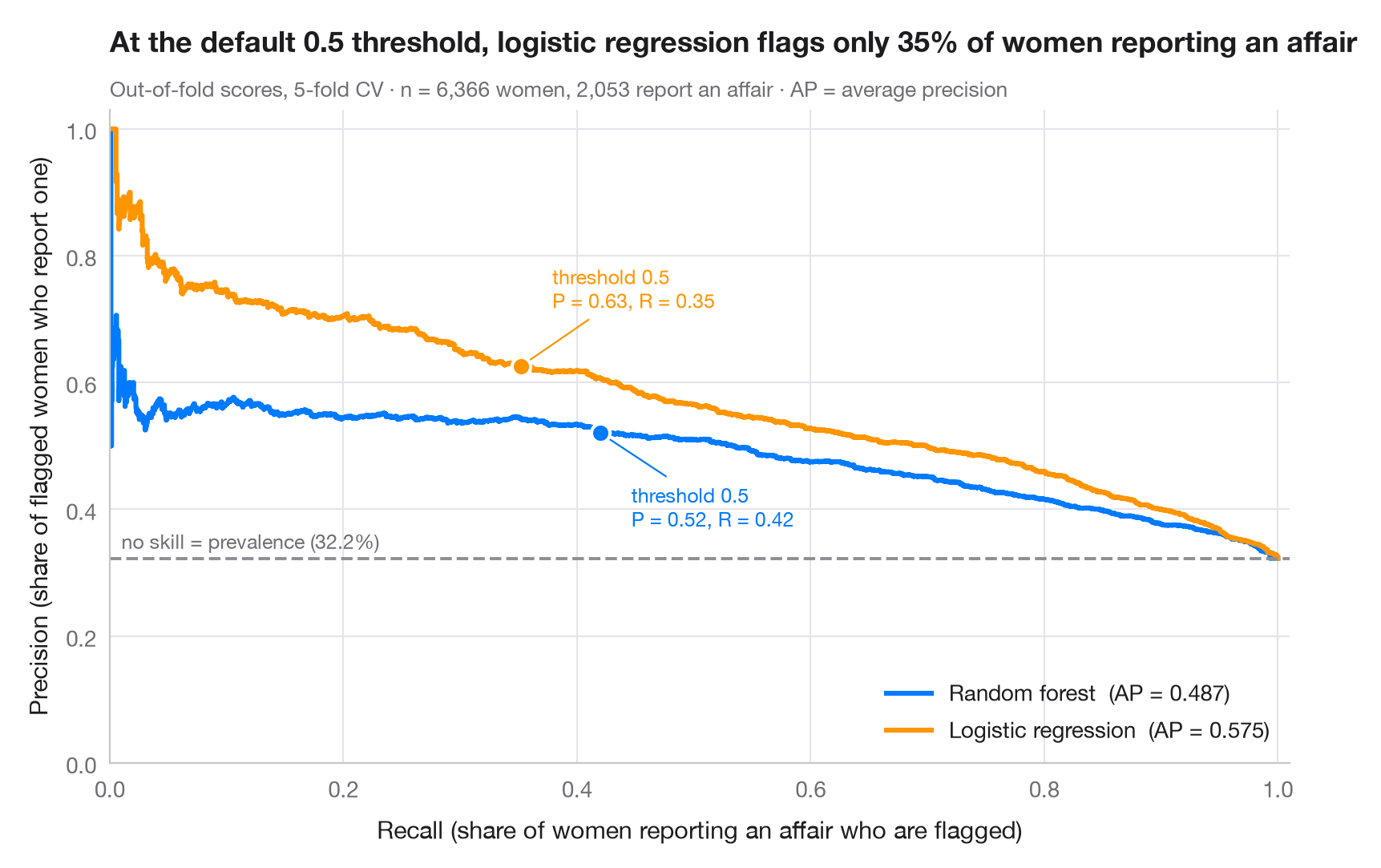
陽性クラスが少数派の場合、ROC 曲線は優れて見えても、警告の多くが誤りということがあります。適合率–再現率曲線は実務上の問いに答えます。陽性のこの割合を見つけたい(再現率)とき、警告のうちどれだけが正しいか(適合率)。各点がひとつの判定しきい値に対応します。破線は無技能のベースライン、すなわち陽性クラスの有病率で、各曲線の下の面積は 平均適合率(AP)で要約されます。
データは、Fair(1978)が分析した 1974 年の Redbook 誌調査の既婚女性 6,366 人で、statsmodels に付属しています(sm.datasets.fair)。目的変数は婚外関係を 1 度でも申告したかどうかで、約 3 人に 1 人という少数派クラスです。予測変数は、結婚生活の評価、年齢、結婚年数、子どもの数、信仰の篤さ、学歴、本人と夫の職業です。スコアは 5 分割交差検証による out-of-fold の確率(cross_val_predict(method="predict_proba"))で、曲線と AP は precision_recall_curve と average_precision_score によります。マーカーは各曲線上の既定のしきい値 0.5 を示します。ここではロジスティック回帰のほうがランダムフォレストより女性をうまく順位づけますが(AP が高い)、しきい値 0.5 では婚外関係を申告した人の約 3 分の 1 しか拾えません。
コードおよび図中のテキストは英語です。
import matplotlib.pyplot as plt
import numpy as np
import statsmodels.api as sm
from sklearn.ensemble import RandomForestClassifier
from sklearn.linear_model import LogisticRegression
from sklearn.metrics import average_precision_score, precision_recall_curve
from sklearn.model_selection import StratifiedKFold, cross_val_predict
from sklearn.pipeline import make_pipeline
from sklearn.preprocessing import StandardScaler

# Data: 6,366 married women (1974 survey); 1 = reports any extramarital affair (a minority class)
d = sm.datasets.fair.load_pandas().data
X = d.drop(columns="affairs")
y = (d["affairs"] > 0).astype(int).to_numpy()
prevalence = y.mean()

models = {
    "Random forest": RandomForestClassifier(n_estimators=300, random_state=0),
    "Logistic regression": make_pipeline(StandardScaler(), LogisticRegression(max_iter=2000)),
}
palette = ["#007AFF", "#FF9500"]
cv = StratifiedKFold(n_splits=5, shuffle=True, random_state=0)
recall = {}

fig, ax = plt.subplots(figsize=(8, 5.2))
for (name, model), c in zip(models.items(), palette):
    score = cross_val_predict(model, X, y, cv=cv, method="predict_proba")[:, 1]
    prec, rec, thr = precision_recall_curve(y, score)
    ap = average_precision_score(y, score)
    ax.step(rec, prec, where="post", color=c, lw=2.2, label=f"{name}  (AP = {ap:.3f})")
    k = np.argmin(np.abs(thr - 0.5))  # the default threshold
    recall[name] = rec[k]
    ax.scatter(rec[k], prec[k], s=70, color=c, edgecolor="white", lw=1.5, zorder=4)
    ax.annotate(f"threshold 0.5\nP = {prec[k]:.2f}, R = {rec[k]:.2f}", (rec[k], prec[k]),
                xytext=(14, -42 if c == palette[0] else 26), textcoords="offset points",
                ha="left", fontsize=9, color=c,
                arrowprops=dict(arrowstyle="-", color=c, lw=0.8))

ax.axhline(prevalence, color="#8E8E93", ls="--", lw=1.4)
ax.text(0.01, prevalence + 0.015, f"no skill = prevalence ({prevalence:.1%})", fontsize=9, color="#6E6E73")
ax.set_xlim(0, 1.01)
ax.set_ylim(0, 1.03)
ax.set_xlabel("Recall (share of women reporting an affair who are flagged)")
ax.set_ylabel("Precision (share of flagged women who report one)")
ax.grid(axis="x")
ax.legend(loc="lower right")
ax.set_title(f"At the default 0.5 threshold, logistic regression flags only {recall['Logistic regression']:.0%} "
             "of women reporting an affair", pad=26)
ax.text(0, 1.02, f"Out-of-fold scores, 5-fold CV · n = {len(y):,} women, {y.sum():,} report an affair · "
        "AP = average precision", transform=ax.transAxes, fontsize=9.5, color="#6E6E73")
plt.show()
図にはオプションの PyStatlas スタイル を使用しています。同じ見た目にするには plt.style.use("pystatlas.mplstyle") を追加してください。
データの出典
- Redbook survey of married women, 1974 (Fair's affairs data). Fair, R. C. (1978). A theory of extramarital affairs. Journal of Political Economy, 86(1), 45–61. https://doi.org/10.1086/260646
Data from the 1974 Redbook magazine survey; distributed with statsmodels (sm.datasets.fair) with the author's permission.
これらの例は統計手法を説明するためのものです。図のタイトルは、この特定のデータ(多くは小規模で、古く、部分的な標本)で図が示す内容を述べたものであり、実質的な問いに対する著者の立場ではありません。解釈、背景、データの質については、ここに挙げた元の出典を参照してください。
引用方法
PyStatlas は Thierry Warin が作成・運営しています。研究や業務に役立った場合は、ぜひ引用してください。
Warin, T. (2026). Precision–recall curves. In PyStatlas: A Python Gallery of Statistical Graphics for the Social Sciences. https://warint.github.io/pystatlas/machine-learning/precision-recall/
@misc{warin2026statlas,
  author       = {Warin, Thierry},
  title        = {PyStatlas: A Python Gallery of Statistical Graphics for the Social Sciences},
  year         = {2026},
  howpublished = {\url{https://warint.github.io/pystatlas/}},
  note         = {Source code: https://github.com/warint/pystatlas}
}機械学習のその他のグラフ
指標付き混同行列
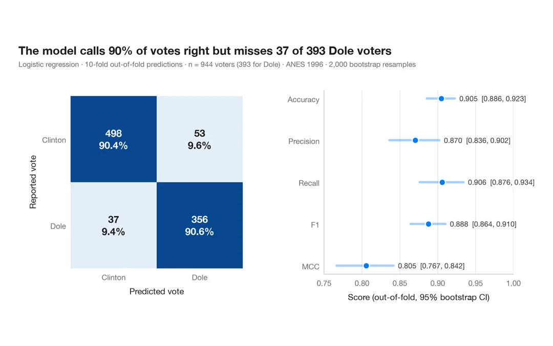
1996 年にドールに投票した人をロジスティック回帰がどれだけ当てられるか。件数と行ごとの割合を示す交差検証の混同行列に、主要指標のブートストラップ区間を添えます。
yardstick::conf_mat() + autoplot()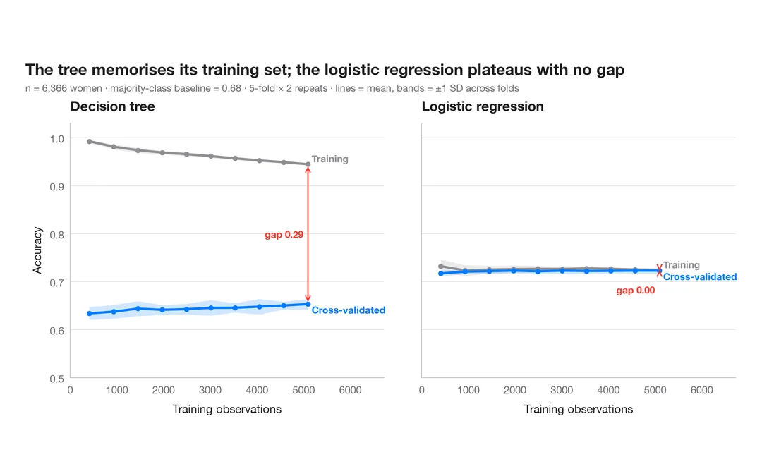
学習曲線
既婚女性のうち誰が婚外関係を申告するかを予測する 2 つのモデルについて、訓練データを増やしたときの訓練正解率と交差検証正解率を示します。
caret::learning_curve_dat() + ggplot()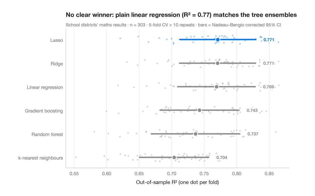
交差検証によるモデル比較
カリフォルニア州の学区の数学の成績を予測する 6 つのモデルの分割ごとの R² を、平均値と補正済み 95% 区間とともに示します。
caret::resamples() + bwplot() / tune::autoplot()