精确率–召回率曲线
两个分类器预测哪些已婚女性报告有婚外情的样本外精确率–召回率曲线,附平均精确率与无技能基线。
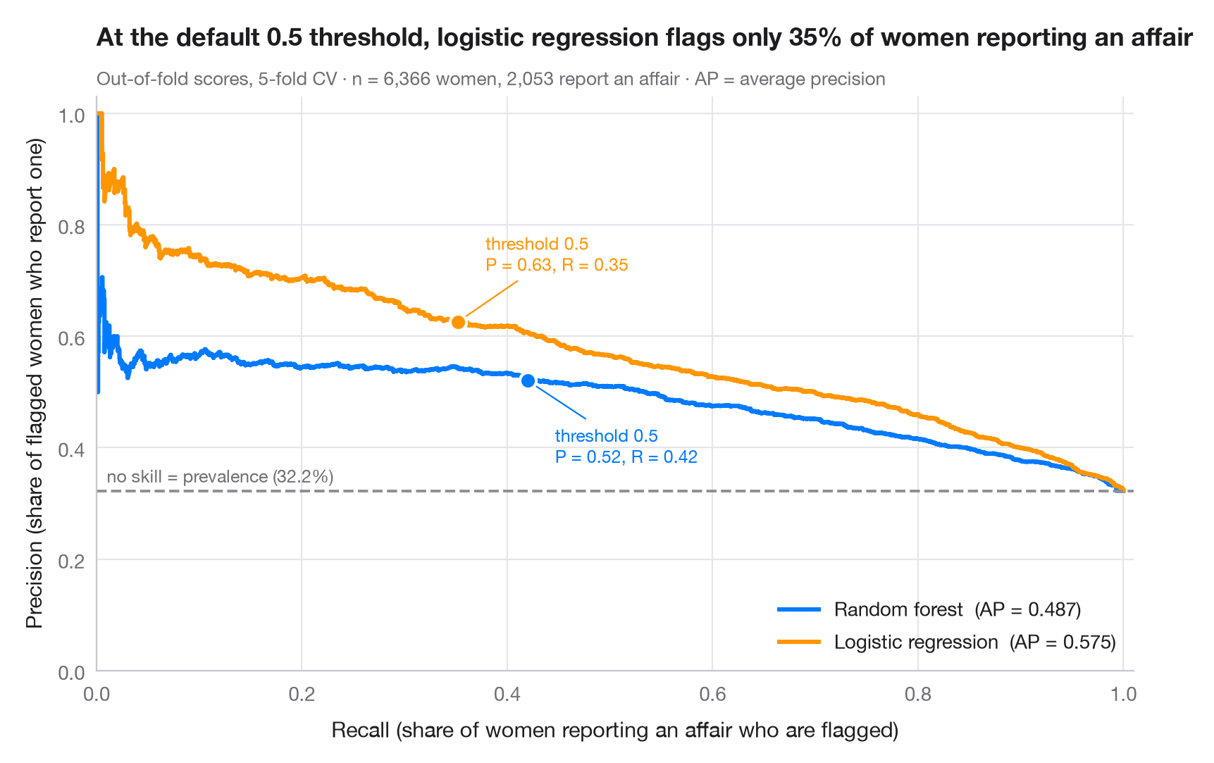
当正类是少数类时,ROC 曲线可能看起来很出色,而许多警报却是误报。精确率–召回率曲线回答的是实际操作中的问题:如果我想找出这一比例的正例(召回率),我的警报中有多少是对的(精确率)?每个点对应一个判定阈值。虚线是无技能基线——即正类的患病率——每条曲线下的面积由 平均精确率(AP)概括。
数据为 Fair(1978)分析的 1974 年《Redbook》杂志调查中的 6,366 名已婚女性,由 statsmodels 提供(sm.datasets.fair)。结果变量为是否报告有过婚外情——一个少数类,约占三分之一。预测变量为她对婚姻的评分、年龄、结婚年数、子女数、宗教虔诚度、教育程度以及她本人和丈夫的职业。得分为 5 折交叉验证的样本外概率(cross_val_predict(method="predict_proba"));曲线和 AP 来自 precision_recall_curve 与 average_precision_score。标记点表示每条曲线上默认的 0.5 阈值。这里逻辑回归对女性的排序优于随机森林(AP 更高),但在 0.5 阈值下,它只标出了约三分之一报告有婚外情的女性。
代码及图中文字均为英文。
import matplotlib.pyplot as plt
import numpy as np
import statsmodels.api as sm
from sklearn.ensemble import RandomForestClassifier
from sklearn.linear_model import LogisticRegression
from sklearn.metrics import average_precision_score, precision_recall_curve
from sklearn.model_selection import StratifiedKFold, cross_val_predict
from sklearn.pipeline import make_pipeline
from sklearn.preprocessing import StandardScaler

# Data: 6,366 married women (1974 survey); 1 = reports any extramarital affair (a minority class)
d = sm.datasets.fair.load_pandas().data
X = d.drop(columns="affairs")
y = (d["affairs"] > 0).astype(int).to_numpy()
prevalence = y.mean()

models = {
    "Random forest": RandomForestClassifier(n_estimators=300, random_state=0),
    "Logistic regression": make_pipeline(StandardScaler(), LogisticRegression(max_iter=2000)),
}
palette = ["#007AFF", "#FF9500"]
cv = StratifiedKFold(n_splits=5, shuffle=True, random_state=0)
recall = {}

fig, ax = plt.subplots(figsize=(8, 5.2))
for (name, model), c in zip(models.items(), palette):
    score = cross_val_predict(model, X, y, cv=cv, method="predict_proba")[:, 1]
    prec, rec, thr = precision_recall_curve(y, score)
    ap = average_precision_score(y, score)
    ax.step(rec, prec, where="post", color=c, lw=2.2, label=f"{name}  (AP = {ap:.3f})")
    k = np.argmin(np.abs(thr - 0.5))  # the default threshold
    recall[name] = rec[k]
    ax.scatter(rec[k], prec[k], s=70, color=c, edgecolor="white", lw=1.5, zorder=4)
    ax.annotate(f"threshold 0.5\nP = {prec[k]:.2f}, R = {rec[k]:.2f}", (rec[k], prec[k]),
                xytext=(14, -42 if c == palette[0] else 26), textcoords="offset points",
                ha="left", fontsize=9, color=c,
                arrowprops=dict(arrowstyle="-", color=c, lw=0.8))

ax.axhline(prevalence, color="#8E8E93", ls="--", lw=1.4)
ax.text(0.01, prevalence + 0.015, f"no skill = prevalence ({prevalence:.1%})", fontsize=9, color="#6E6E73")
ax.set_xlim(0, 1.01)
ax.set_ylim(0, 1.03)
ax.set_xlabel("Recall (share of women reporting an affair who are flagged)")
ax.set_ylabel("Precision (share of flagged women who report one)")
ax.grid(axis="x")
ax.legend(loc="lower right")
ax.set_title(f"At the default 0.5 threshold, logistic regression flags only {recall['Logistic regression']:.0%} "
             "of women reporting an affair", pad=26)
ax.text(0, 1.02, f"Out-of-fold scores, 5-fold CV · n = {len(y):,} women, {y.sum():,} report an affair · "
        "AP = average precision", transform=ax.transAxes, fontsize=9.5, color="#6E6E73")
plt.show()
图表使用了可选的 PyStatlas 样式:添加 plt.style.use("pystatlas.mplstyle") 即可完全还原其外观。
数据来源
- Redbook survey of married women, 1974 (Fair's affairs data). Fair, R. C. (1978). A theory of extramarital affairs. Journal of Political Economy, 86(1), 45–61. https://doi.org/10.1086/260646
Data from the 1974 Redbook magazine survey; distributed with statsmodels (sm.datasets.fair) with the author's permission.
这些示例用于说明统计方法。图表标题描述的是该图在这些特定数据中呈现的内容——这些数据往往样本较小、年代较早或并不完整——而不是作者对实质问题的立场。关于解释、背景和数据质量,请以此处引用的原始来源为准。
如何引用
PyStatlas 由 Thierry Warin 创建并维护。如果它对你的工作有所帮助,敬请引用。
Warin, T. (2026). Precision–recall curves. In PyStatlas: A Python Gallery of Statistical Graphics for the Social Sciences. https://warint.github.io/pystatlas/machine-learning/precision-recall/
@misc{warin2026statlas,
  author       = {Warin, Thierry},
  title        = {PyStatlas: A Python Gallery of Statistical Graphics for the Social Sciences},
  year         = {2026},
  howpublished = {\url{https://warint.github.io/pystatlas/}},
  note         = {Source code: https://github.com/warint/pystatlas}
}