带指标的混淆矩阵
逻辑回归能多好地预测谁在 1996 年投票给多尔——样本外混淆矩阵,显示计数与行内占比,并为主要指标给出自助法区间。
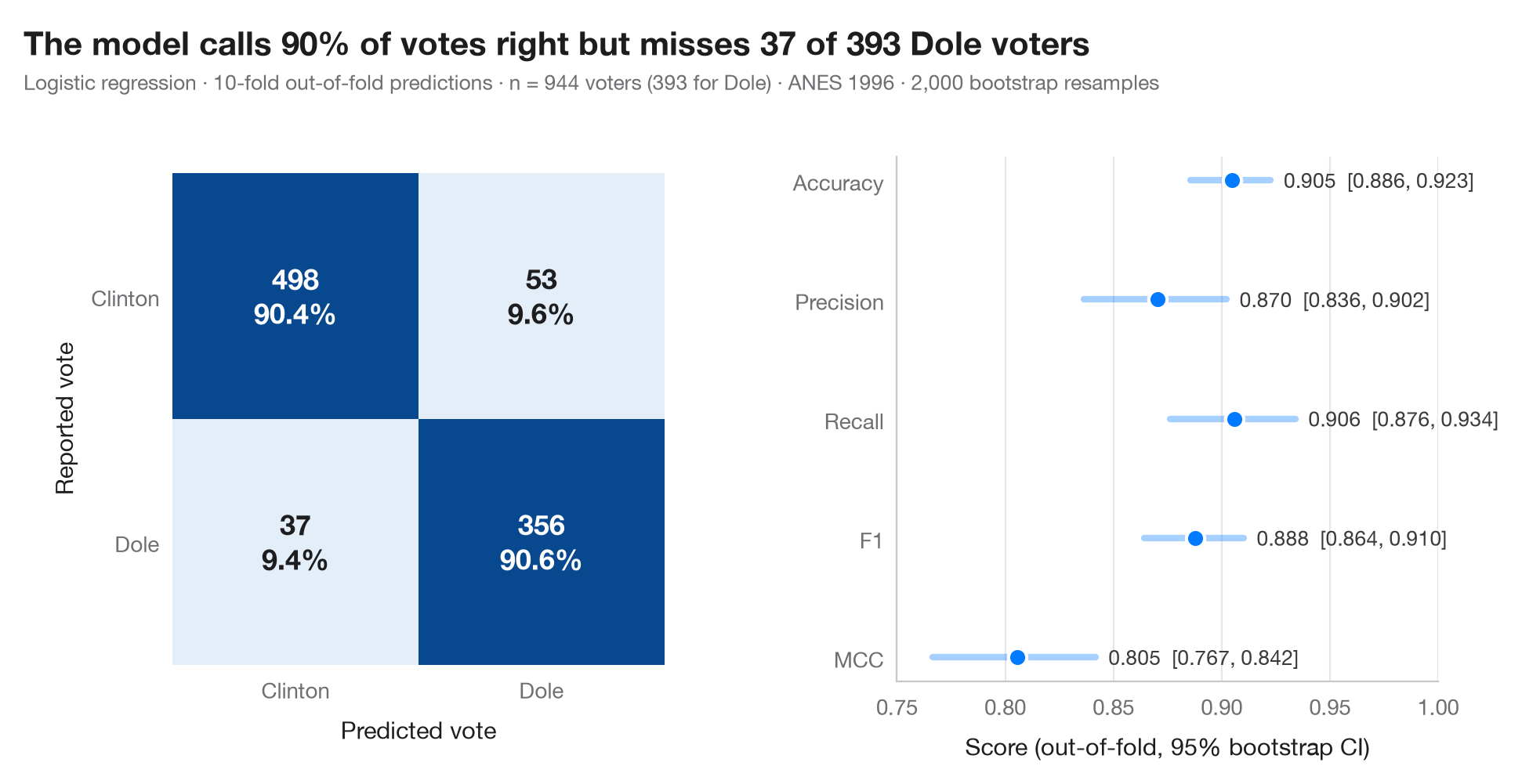
混淆矩阵将真实类别与预测类别交叉列出。每个格子显示计数及其在真实类别(行)中的占比,因此对角线可直接读作灵敏度和特异度。预测为 样本外(out-of-fold) 预测:在 10 折交叉验证中,每个观测都由一个从未见过它的模型来预测——这正是矩阵在新数据上的样子。
右侧面板给出准确率、精确率、召回率、F1 和马修斯相关系数(MCC),每项都附有 95% 自助法区间:单个数字掩盖了换一个样本时它会变动多少。数据为 statsmodels 自带的 1996 年美国全国选举研究(ANES)中投票给克林顿或多尔的 944 名受访者(sm.datasets.anes96)。模型根据政党认同、左右自我定位、年龄、教育程度、收入、收看电视新闻的天数以及居住地人口(对数)预测是否投票给多尔。模型为标准化的逻辑回归;预测来自 cross_val_predict,指标来自 sklearn.metrics。
代码及图中文字均为英文。
import matplotlib.pyplot as plt
import numpy as np
import statsmodels.api as sm
from sklearn.linear_model import LogisticRegression
from sklearn.metrics import (accuracy_score, confusion_matrix, f1_score, matthews_corrcoef,
                             precision_score, recall_score)
from sklearn.model_selection import StratifiedKFold, cross_val_predict
from sklearn.pipeline import make_pipeline
from sklearn.preprocessing import StandardScaler

# Data: 944 voters in the 1996 US presidential election; 1 = voted Dole, 0 = voted Clinton
d = sm.datasets.anes96.load_pandas().data
X = d[["PID", "selfLR", "age", "educ", "income", "TVnews", "logpopul"]]
y = d["vote"].to_numpy().astype(int)
labels = ["Clinton", "Dole"]

# Out-of-fold predictions from a 10-fold cross-validation
model = make_pipeline(StandardScaler(), LogisticRegression(max_iter=1000))
cv = StratifiedKFold(n_splits=10, shuffle=True, random_state=0)
pred = cross_val_predict(model, X, y, cv=cv)
cm = confusion_matrix(y, pred)

# Metrics with 95% bootstrap intervals
metrics = {"Accuracy": accuracy_score, "Precision": precision_score, "Recall": recall_score,
           "F1": f1_score, "MCC": matthews_corrcoef}
rng = np.random.default_rng(1)
boot = {k: [] for k in metrics}
for _ in range(2000):
    i = rng.integers(0, len(y), len(y))
    for k, f in metrics.items():
        boot[k].append(f(y[i], pred[i]))
point = {k: f(y, pred) for k, f in metrics.items()}
ci = {k: np.percentile(v, [2.5, 97.5]) for k, v in boot.items()}

plt.rcParams["figure.constrained_layout.use"] = False   # manual margins leave room for the subtitle
fig, (ax, axm) = plt.subplots(1, 2, figsize=(9.5, 5), gridspec_kw=dict(width_ratios=(1, 1.1)))
fig.subplots_adjust(left=0.12, right=0.97, top=0.80, bottom=0.13, wspace=0.45)

# Confusion matrix: colour = share of the true class
share = cm / cm.sum(axis=1, keepdims=True)
ax.imshow(share, cmap="Blues", vmin=0, vmax=1)
for r in range(2):
    for c in range(2):
        ax.text(c, r, f"{cm[r, c]}\n{share[r, c]:.1%}", ha="center", va="center", fontsize=13,
                fontweight="semibold", color="white" if share[r, c] > 0.5 else "#1d1d1f")
ax.set_xticks([0, 1], labels)
ax.set_yticks([0, 1], labels)
ax.set_xlabel("Predicted vote")
ax.set_ylabel("Reported vote")
ax.grid(False)
for s in ax.spines.values():
    s.set_visible(False)

# Metrics with intervals
names = list(metrics)[::-1]
for j, k in enumerate(names):
    axm.plot(ci[k], [j, j], color="#007AFF", lw=3, solid_capstyle="round", alpha=0.35)
    axm.scatter(point[k], j, s=70, color="#007AFF", zorder=3, edgecolor="white", lw=1.5)
    axm.text(ci[k][1] + 0.006, j, f"{point[k]:.3f}  [{ci[k][0]:.3f}, {ci[k][1]:.3f}]",
             va="center", fontsize=9.5, color="#3A3A3C")
axm.set_yticks(range(len(names)), names)
axm.set_xlim(0.75, 1.0)
axm.set_xlabel("Score (out-of-fold, 95% bootstrap CI)")
axm.grid(axis="x"); axm.grid(axis="y", visible=False)

fn, pos = cm[1, 0], cm[1].sum()
fig.suptitle(f"The model calls {point['Accuracy']:.0%} of votes right but misses {fn} of {pos} Dole voters",
             x=0.02, y=0.97, ha="left")
fig.text(0.02, 0.885, f"Logistic regression · 10-fold out-of-fold predictions · n = {len(y)} voters "
         f"({y.sum()} for Dole) · ANES 1996 · 2,000 bootstrap resamples", fontsize=9.5, color="#6E6E73")
plt.show()
图表使用了可选的 PyStatlas 样式:添加 plt.style.use("pystatlas.mplstyle") 即可完全还原其外观。
数据来源
- American National Election Study, 1996. Rosenstone, S. J., Kinder, D. R., Miller, W. E., & the National Election Studies. (2016). ANES 1996 Time Series Study (ICPSR 6896; Version 6) [Data set]. Inter-university Consortium for Political and Social Research. https://doi.org/10.3886/ICPSR06896.v6
Subset of 944 respondents distributed with statsmodels (sm.datasets.anes96); public domain.
这些示例用于说明统计方法。图表标题描述的是该图在这些特定数据中呈现的内容——这些数据往往样本较小、年代较早或并不完整——而不是作者对实质问题的立场。关于解释、背景和数据质量,请以此处引用的原始来源为准。
如何引用
PyStatlas 由 Thierry Warin 创建并维护。如果它对你的工作有所帮助,敬请引用。
Warin, T. (2026). Confusion matrix with metrics. In PyStatlas: A Python Gallery of Statistical Graphics for the Social Sciences. https://warint.github.io/pystatlas/machine-learning/confusion-matrix/
@misc{warin2026statlas,
  author       = {Warin, Thierry},
  title        = {PyStatlas: A Python Gallery of Statistical Graphics for the Social Sciences},
  year         = {2026},
  howpublished = {\url{https://warint.github.io/pystatlas/}},
  note         = {Source code: https://github.com/warint/pystatlas}
}