指標付き混同行列
1996 年にドールに投票した人をロジスティック回帰がどれだけ当てられるか。件数と行ごとの割合を示す交差検証の混同行列に、主要指標のブートストラップ区間を添えます。
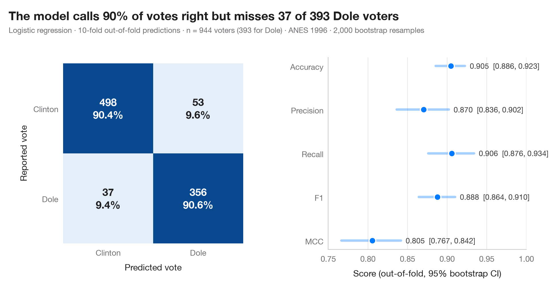
混同行列は、実際のクラスと予測されたクラスを掛け合わせた表です。各セルには件数と、その実際のクラス(行)に占める割合を示すので、対角線はそのまま感度と特異度として読めます。予測は out-of-fold(交差検証の検証側) の予測です。各観測値は、10 分割交差検証の中でその観測値を一度も見ていないモデルによって予測されます。つまり、新しいデータに対する混同行列の姿です。
右のパネルには、正解率、適合率、再現率、F1、マシューズ相関係数(MCC)を、それぞれ 95% ブートストラップ区間とともに示します。数値ひとつだけでは、別の標本でどれほど動くかが分かりません。データは statsmodels 付属の 1996 年米国全国選挙調査(ANES)で、クリントンかドールに投票した回答者 944 人です(sm.datasets.anes96)。モデルは、支持政党、左右の自己位置づけ、年齢、学歴、所得、テレビニュースを見る日数、居住地の人口(対数)からドールへの投票を予測します。モデルは標準化したロジスティック回帰で、予測は cross_val_predict、指標は sklearn.metrics によります。
コードおよび図中のテキストは英語です。
import matplotlib.pyplot as plt
import numpy as np
import statsmodels.api as sm
from sklearn.linear_model import LogisticRegression
from sklearn.metrics import (accuracy_score, confusion_matrix, f1_score, matthews_corrcoef,
                             precision_score, recall_score)
from sklearn.model_selection import StratifiedKFold, cross_val_predict
from sklearn.pipeline import make_pipeline
from sklearn.preprocessing import StandardScaler

# Data: 944 voters in the 1996 US presidential election; 1 = voted Dole, 0 = voted Clinton
d = sm.datasets.anes96.load_pandas().data
X = d[["PID", "selfLR", "age", "educ", "income", "TVnews", "logpopul"]]
y = d["vote"].to_numpy().astype(int)
labels = ["Clinton", "Dole"]

# Out-of-fold predictions from a 10-fold cross-validation
model = make_pipeline(StandardScaler(), LogisticRegression(max_iter=1000))
cv = StratifiedKFold(n_splits=10, shuffle=True, random_state=0)
pred = cross_val_predict(model, X, y, cv=cv)
cm = confusion_matrix(y, pred)

# Metrics with 95% bootstrap intervals
metrics = {"Accuracy": accuracy_score, "Precision": precision_score, "Recall": recall_score,
           "F1": f1_score, "MCC": matthews_corrcoef}
rng = np.random.default_rng(1)
boot = {k: [] for k in metrics}
for _ in range(2000):
    i = rng.integers(0, len(y), len(y))
    for k, f in metrics.items():
        boot[k].append(f(y[i], pred[i]))
point = {k: f(y, pred) for k, f in metrics.items()}
ci = {k: np.percentile(v, [2.5, 97.5]) for k, v in boot.items()}

plt.rcParams["figure.constrained_layout.use"] = False   # manual margins leave room for the subtitle
fig, (ax, axm) = plt.subplots(1, 2, figsize=(9.5, 5), gridspec_kw=dict(width_ratios=(1, 1.1)))
fig.subplots_adjust(left=0.12, right=0.97, top=0.80, bottom=0.13, wspace=0.45)

# Confusion matrix: colour = share of the true class
share = cm / cm.sum(axis=1, keepdims=True)
ax.imshow(share, cmap="Blues", vmin=0, vmax=1)
for r in range(2):
    for c in range(2):
        ax.text(c, r, f"{cm[r, c]}\n{share[r, c]:.1%}", ha="center", va="center", fontsize=13,
                fontweight="semibold", color="white" if share[r, c] > 0.5 else "#1d1d1f")
ax.set_xticks([0, 1], labels)
ax.set_yticks([0, 1], labels)
ax.set_xlabel("Predicted vote")
ax.set_ylabel("Reported vote")
ax.grid(False)
for s in ax.spines.values():
    s.set_visible(False)

# Metrics with intervals
names = list(metrics)[::-1]
for j, k in enumerate(names):
    axm.plot(ci[k], [j, j], color="#007AFF", lw=3, solid_capstyle="round", alpha=0.35)
    axm.scatter(point[k], j, s=70, color="#007AFF", zorder=3, edgecolor="white", lw=1.5)
    axm.text(ci[k][1] + 0.006, j, f"{point[k]:.3f}  [{ci[k][0]:.3f}, {ci[k][1]:.3f}]",
             va="center", fontsize=9.5, color="#3A3A3C")
axm.set_yticks(range(len(names)), names)
axm.set_xlim(0.75, 1.0)
axm.set_xlabel("Score (out-of-fold, 95% bootstrap CI)")
axm.grid(axis="x"); axm.grid(axis="y", visible=False)

fn, pos = cm[1, 0], cm[1].sum()
fig.suptitle(f"The model calls {point['Accuracy']:.0%} of votes right but misses {fn} of {pos} Dole voters",
             x=0.02, y=0.97, ha="left")
fig.text(0.02, 0.885, f"Logistic regression · 10-fold out-of-fold predictions · n = {len(y)} voters "
         f"({y.sum()} for Dole) · ANES 1996 · 2,000 bootstrap resamples", fontsize=9.5, color="#6E6E73")
plt.show()
図にはオプションの PyStatlas スタイル を使用しています。同じ見た目にするには plt.style.use("pystatlas.mplstyle") を追加してください。
データの出典
- American National Election Study, 1996. Rosenstone, S. J., Kinder, D. R., Miller, W. E., & the National Election Studies. (2016). ANES 1996 Time Series Study (ICPSR 6896; Version 6) [Data set]. Inter-university Consortium for Political and Social Research. https://doi.org/10.3886/ICPSR06896.v6
Subset of 944 respondents distributed with statsmodels (sm.datasets.anes96); public domain.
これらの例は統計手法を説明するためのものです。図のタイトルは、この特定のデータ(多くは小規模で、古く、部分的な標本)で図が示す内容を述べたものであり、実質的な問いに対する著者の立場ではありません。解釈、背景、データの質については、ここに挙げた元の出典を参照してください。
引用方法
PyStatlas は Thierry Warin が作成・運営しています。研究や業務に役立った場合は、ぜひ引用してください。
Warin, T. (2026). Confusion matrix with metrics. In PyStatlas: A Python Gallery of Statistical Graphics for the Social Sciences. https://warint.github.io/pystatlas/machine-learning/confusion-matrix/
@misc{warin2026statlas,
  author       = {Warin, Thierry},
  title        = {PyStatlas: A Python Gallery of Statistical Graphics for the Social Sciences},
  year         = {2026},
  howpublished = {\url{https://warint.github.io/pystatlas/}},
  note         = {Source code: https://github.com/warint/pystatlas}
}機械学習のその他のグラフ
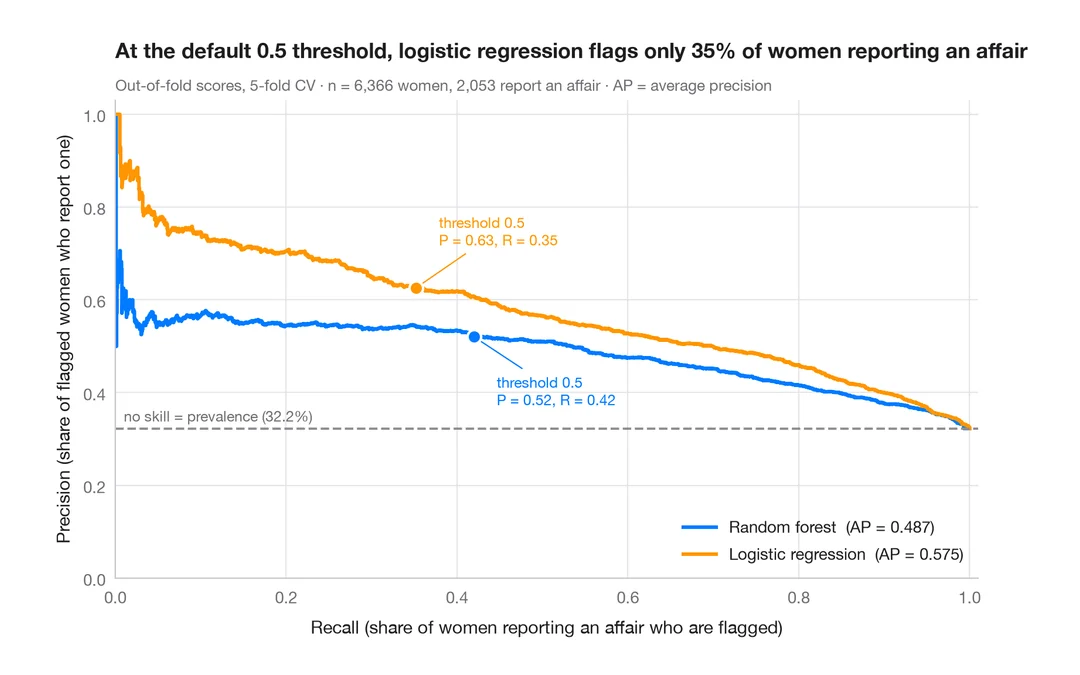
適合率–再現率曲線
既婚女性のうち誰が婚外関係を申告するかを予測する 2 つの分類器の、交差検証による適合率–再現率曲線と、平均適合率、無技能のベースライン。
yardstick::pr_curve() + autoplot()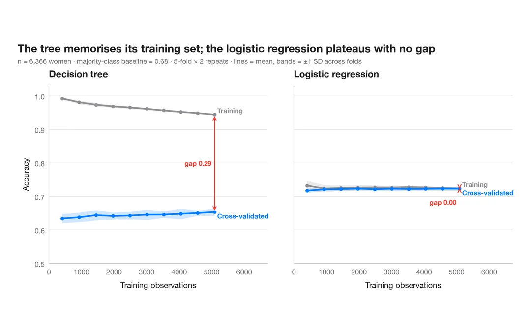
学習曲線
既婚女性のうち誰が婚外関係を申告するかを予測する 2 つのモデルについて、訓練データを増やしたときの訓練正解率と交差検証正解率を示します。
caret::learning_curve_dat() + ggplot()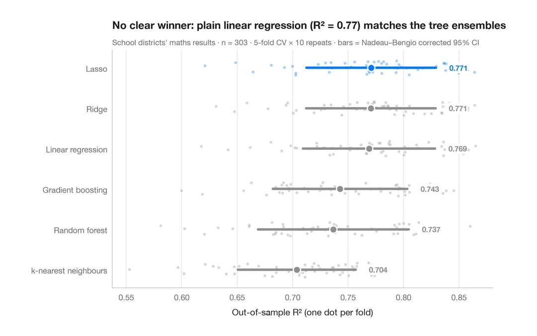
交差検証によるモデル比較
カリフォルニア州の学区の数学の成績を予測する 6 つのモデルの分割ごとの R² を、平均値と補正済み 95% 区間とともに示します。
caret::resamples() + bwplot() / tune::autoplot()