Bland–Altman plot
Do two coders place party manifestos on the left–right scale the same way? Bias and 95% limits of agreement.
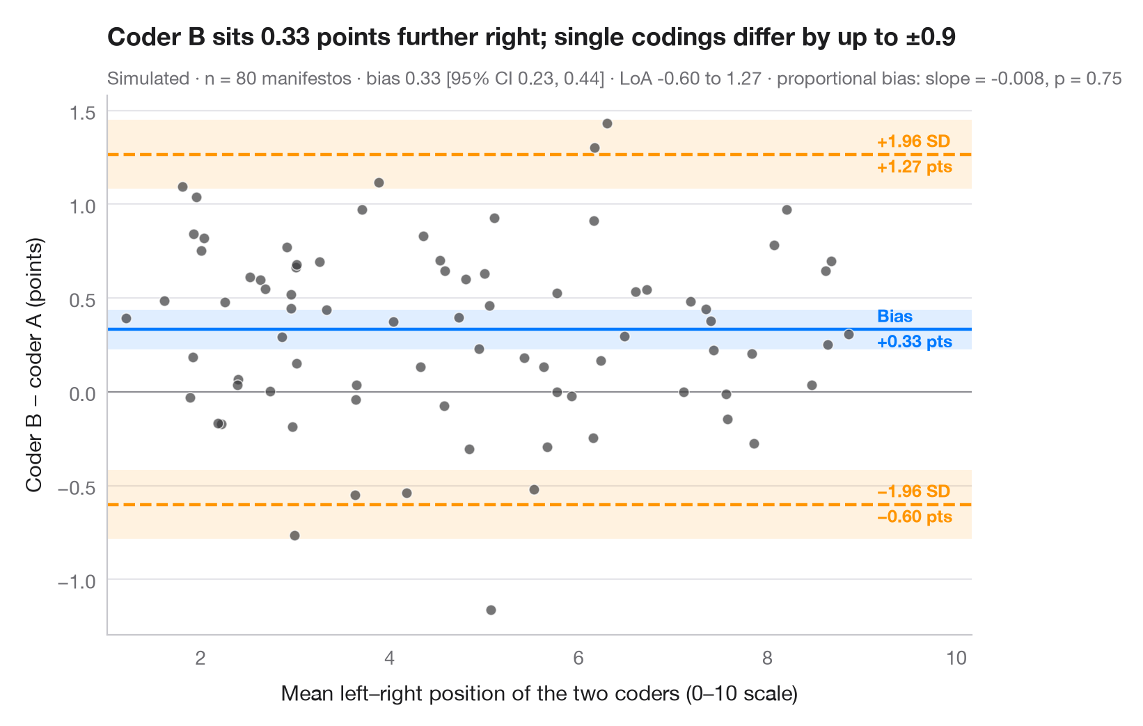
When two instruments — or two coders — measure the same thing, a high correlation says nothing about whether they agree. The Bland–Altman plot puts the difference between methods on the y-axis and their average on the x-axis. The middle line is the mean difference (systematic bias), the outer lines the 95% limits of agreement (bias ± 1.96 SD) within which most disagreements fall. Shaded bands are the 95% confidence intervals of these three lines, using the Bland & Altman (1986) standard errors; a slope in the cloud would signal a proportional bias.
Data are simulated with numpy (seeded) to mimic a classic
content-analysis check: two trained coders each place the same 80 party
manifestos on a 0–10 left–right scale, and coder B is built to sit about 0.4
points to the right of coder A. Bias and intervals use scipy.stats.t; the
slope test is an OLS fit from statsmodels.
import matplotlib.pyplot as plt
import numpy as np
import statsmodels.api as sm
from scipy import stats

# Simulated coding: 80 manifestos placed on a 0–10 left–right scale by two coders;
# coder B leans ~0.4 points to the right and is a little noisier
rng = np.random.default_rng(11)
n = 80
position = rng.uniform(1.5, 8.5, n)
coder_a = position + rng.normal(0, 0.35, n)
coder_b = position + 0.4 + rng.normal(0, 0.45, n)

mean, diff = (coder_a + coder_b) / 2, coder_b - coder_a
bias, sd = diff.mean(), diff.std(ddof=1)
loa = bias + np.array([-1.96, 1.96]) * sd
t = stats.t.ppf(0.975, n - 1)
ci_bias = t * sd / np.sqrt(n)            # half-width of the CI for the bias
ci_loa = t * np.sqrt(3 * sd**2 / n)      # Bland & Altman (1986) SE of a limit
slope = sm.OLS(diff, sm.add_constant(mean)).fit()

fig, ax = plt.subplots(figsize=(8, 5))
for y0, hw, c in [(bias, ci_bias, "#007AFF"), (loa[0], ci_loa, "#FF9500"), (loa[1], ci_loa, "#FF9500")]:
    ax.axhspan(y0 - hw, y0 + hw, color=c, alpha=0.12, lw=0)
    ax.axhline(y0, color=c, lw=1.6, ls="-" if c == "#007AFF" else "--")
ax.axhline(0, color="#8E8E93", lw=0.8)
ax.scatter(mean, diff, s=30, color="#3A3A3C", alpha=0.7, edgecolor="white", lw=0.6, zorder=3)

# Labels on the right margin
x_lab = mean.max() + 0.3
for y0, name, c in [(loa[1], "+1.96 SD", "#FF9500"), (bias, "Bias", "#007AFF"),
                    (loa[0], "−1.96 SD", "#FF9500")]:
    ax.text(x_lab, y0, f"{name}\n{y0:+.2f} pts".replace("-", "−"), va="center", ha="left", fontsize=9,
            color=c, fontweight="semibold", linespacing=1.3)

ax.set_xlim(mean.min() - 0.2, mean.max() + 1.3)
ax.set_xlabel("Mean left–right position of the two coders (0–10 scale)")
ax.set_ylabel("Coder B − coder A (points)")
ax.set_title(f"Coder B sits {bias:.2f} points further right; single codings differ "
             f"by up to ±{1.96 * sd:.1f}", pad=26)
ax.text(0, 1.02, f"Simulated · n = {n} manifestos · bias {bias:.2f} [95% CI {bias - ci_bias:.2f}, "
        f"{bias + ci_bias:.2f}] · LoA {loa[0]:.2f} to {loa[1]:.2f} · proportional bias: slope = {slope.params[1]:.3f}, "
        f"p = {slope.pvalues[1]:.2f}", transform=ax.transAxes, fontsize=9.5, color="#6E6E73")
plt.show()
Figures use the optional PyStatlas style: add plt.style.use("pystatlas.mplstyle") to match the look exactly.
Data source
- Simulated data. Simulated data with a fixed random seed, created for this example.
No real respondents, documents or measurements: the numbers only illustrate how the chart and its statistics work.
The examples illustrate statistical methods. Their titles describe what each figure shows in these particular data — often a small, dated or partial sample — not the author's position on the substantive question. For interpretation, context and data quality, rely on the original sources cited here.
How to cite
PyStatlas is created and maintained by Thierry Warin. If it helped your work, please cite it.
Warin, T. (2026). Bland–Altman plot. In PyStatlas: A Python Gallery of Statistical Graphics for the Social Sciences. https://warint.github.io/pystatlas/inference-uncertainty/bland-altman/
@misc{warin2026statlas,
  author       = {Warin, Thierry},
  title        = {PyStatlas: A Python Gallery of Statistical Graphics for the Social Sciences},
  year         = {2026},
  howpublished = {\url{https://warint.github.io/pystatlas/}},
  note         = {Source code: https://github.com/warint/pystatlas}
}More in Inference & uncertainty
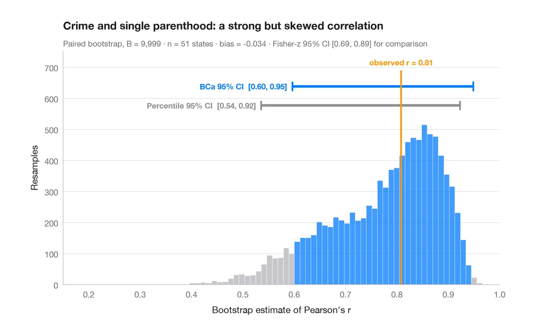
Bootstrap distribution
Resampled correlation with percentile and BCa 95% confidence intervals.
boot::boot() + boot::boot.ci()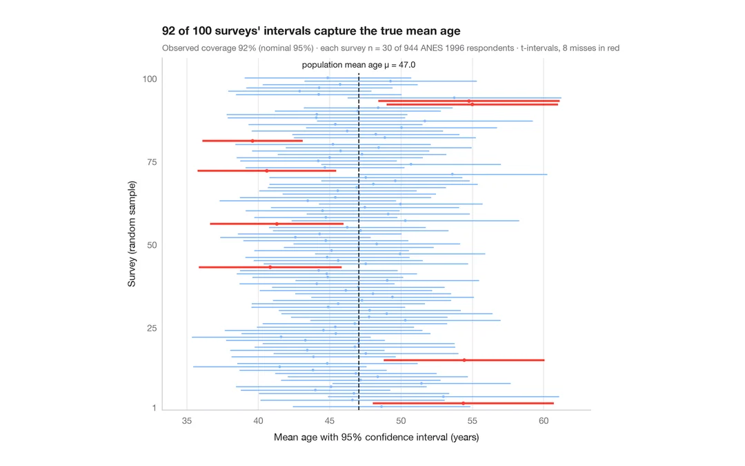
What a 95% confidence interval means
100 surveys of 30 people drawn from 944 ANES respondents; the 95% CIs for mean age that miss the true value are in red.
teaching classic (e.g. TeachingDemos::ci.examp())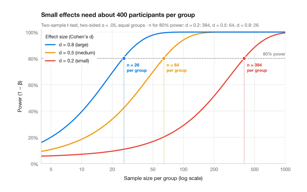
Power curve
Power of a two-sample t-test against sample size for small, medium and large effects.
pwr::pwr.t.test() + plot()