Meta-analysis forest plot
Do teacher expectations raise pupils' IQ? 19 "Pygmalion" experiments, a random-effects pooled diamond and heterogeneity statistics.
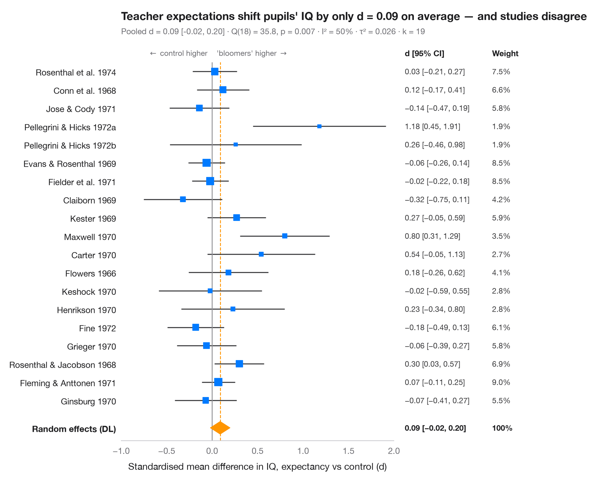
A forest plot lays out every study of a meta-analysis on one line: the square is the study's estimate (its area proportional to the study's weight), the whisker its 95% confidence interval. The diamond at the bottom is the pooled random-effects estimate (DerSimonian–Laird), whose width is its 95% CI. The subtitle reports heterogeneity — Cochran's Q, I² (share of variability due to real between-study differences) and τ² (their variance).
Data are the 19 teacher-expectancy ("Pygmalion") experiments synthesised by
Raudenbush (1984): in each, teachers were told that some pupils were about to
"bloom", and pupils' IQ was later compared with that of a control group. The
effect sizes are standardised mean differences (d > 0: the "bloomers" scored
higher) and their sampling variances, typed in as published in
dat.raudenbush1985 of R's metafor. Pooling uses combine_effects from
statsmodels.stats.meta_analysis. The average effect is small and its CI
includes zero, while the studies vary more than chance allows; Raudenbush
traced much of that variation to how long teachers had known their pupils
before the expectancy was induced.
import matplotlib.pyplot as plt
import numpy as np
import pandas as pd
from matplotlib.transforms import blended_transform_factory
from scipy import stats
from statsmodels.stats.meta_analysis import combine_effects

# Teacher-expectancy experiments (Raudenbush, 1984): standardised mean difference
# in pupil IQ (yi) and its sampling variance (vi), as in metafor's dat.raudenbush1985
pyg = pd.DataFrame({
    "study": ["Rosenthal et al. 1974", "Conn et al. 1968", "Jose & Cody 1971",
              "Pellegrini & Hicks 1972a", "Pellegrini & Hicks 1972b", "Evans & Rosenthal 1969",
              "Fielder et al. 1971", "Claiborn 1969", "Kester 1969", "Maxwell 1970", "Carter 1970",
              "Flowers 1966", "Keshock 1970", "Henrikson 1970", "Fine 1972", "Grieger 1970",
              "Rosenthal & Jacobson 1968", "Fleming & Anttonen 1971", "Ginsburg 1970"],
    "yi": [0.03, 0.12, -0.14, 1.18, 0.26, -0.06, -0.02, -0.32, 0.27, 0.80, 0.54, 0.18, -0.02,
           0.23, -0.18, -0.06, 0.30, 0.07, -0.07],
    "vi": [0.0156, 0.0216, 0.0279, 0.1391, 0.1362, 0.0106, 0.0106, 0.0484, 0.0269, 0.0630,
           0.0912, 0.0497, 0.0835, 0.0841, 0.0253, 0.0279, 0.0193, 0.0088, 0.0303]})
res = combine_effects(pyg.yi, pyg.vi, method_re="dl", row_names=pyg.study)
tab = res.summary_frame()
studies, pooled = tab.iloc[:len(pyg)], tab.loc["random effect"]
q_p = stats.chi2.sf(res.q, res.df_resid)

fig, ax = plt.subplots(figsize=(8, 7.6))
y = np.arange(len(pyg), 0, -1) + 1.0
ax.hlines(y, studies.ci_low, studies.ci_upp, color="#3A3A3C", lw=1.2)
ax.scatter(studies.eff, y, marker="s", s=900 * studies.w_re, color="#007AFF", zorder=3)

# Pooled random-effects diamond
lo, mid, hi = pooled.ci_low, pooled.eff, pooled.ci_upp
ax.fill([lo, mid, hi, mid], [0.5, 0.85, 0.5, 0.15], color="#FF9500", zorder=3)
ax.vlines(0, -0.2, len(pyg) + 1.5, color="#8E8E93", lw=1)
ax.vlines(mid, -0.2, len(pyg) + 1.5, color="#FF9500", lw=1, ls="--", zorder=1)

# Table columns to the right of the plot: d [95% CI] and weight
tr = blended_transform_factory(ax.transAxes, ax.transData)
for x, head in [(1.04, "d [95% CI]"), (1.36, "Weight")]:
    ax.text(x, len(pyg) + 2, head, transform=tr, fontsize=9.5, fontweight="semibold", va="center")
for yi, (_, r) in zip(y, studies.iterrows()):
    ax.text(1.04, yi, f"{r.eff:.2f} [{r.ci_low:.2f}, {r.ci_upp:.2f}]".replace("-", "−"),
            transform=tr, fontsize=9, va="center", color="#3A3A3C")
    ax.text(1.36, yi, f"{100 * r.w_re:.1f}%", transform=tr, fontsize=9, va="center", color="#3A3A3C")
for x, txt in [(1.04, f"{mid:.2f} [{lo:.2f}, {hi:.2f}]".replace("-", "−")), (1.36, "100%")]:
    ax.text(x, 0.5, txt, transform=tr, fontsize=9, va="center", fontweight="semibold")

ax.set_xlim(-1.0, 2.0)
ax.set_yticks(list(y) + [0.5], list(pyg.study) + ["Random effects (DL)"])
ax.get_yticklabels()[-1].set_fontweight("semibold")
ax.set_ylim(-0.2, len(pyg) + 2.6)
ax.grid(False); ax.spines["left"].set_visible(False)
ax.set_xlabel("Standardised mean difference in IQ, expectancy vs control (d)")
ax.text(-0.05, len(pyg) + 2, r"$\leftarrow$ control higher", ha="right", va="center", fontsize=9, color="#6E6E73")
ax.text(0.05, len(pyg) + 2, r"'bloomers' higher $\rightarrow$", ha="left", va="center", fontsize=9, color="#6E6E73")
ax.tick_params(axis="y", labelcolor="#1D1D1F")
ax.set_title(f"Teacher expectations shift pupils' IQ by only d = {mid:.2f} on average — "
             "and studies disagree", pad=26)
ax.text(0, 1.02, f"Pooled d = {mid:.2f} [{lo:.2f}, {hi:.2f}] · Q({res.df_resid:.0f}) = "
        f"{res.q:.1f}, p = {q_p:.3f} · I² = {100 * res.i2:.0f}% · τ² = {res.tau2:.3f} · k = {len(pyg)}",
        transform=ax.transAxes, fontsize=9.5, color="#6E6E73")
plt.show()
Figures use the optional PyStatlas style: add plt.style.use("pystatlas.mplstyle") to match the look exactly.
Data source
- Teacher-expectancy experiments (Raudenbush, 1984). Raudenbush, S. W. (1984). Magnitude of teacher expectancy effects on pupil IQ as a function of the credibility of expectancy induction: A synthesis of findings from 18 experiments. Journal of Educational Psychology, 76(1), 85–97. https://doi.org/10.1037/0022-0663.76.1.85
Effect sizes and variances typed in from dat.raudenbush1985 in R's metadat/metafor (Viechtbauer, 2010, Journal of Statistical Software, 36(3), https://doi.org/10.18637/jss.v036.i03); one of the 18 experiments contributes two rows.
The examples illustrate statistical methods. Their titles describe what each figure shows in these particular data — often a small, dated or partial sample — not the author's position on the substantive question. For interpretation, context and data quality, rely on the original sources cited here.
How to cite
PyStatlas is created and maintained by Thierry Warin. If it helped your work, please cite it.
Warin, T. (2026). Meta-analysis forest plot. In PyStatlas: A Python Gallery of Statistical Graphics for the Social Sciences. https://warint.github.io/pystatlas/inference-uncertainty/meta-analysis-forest/
@misc{warin2026statlas,
  author       = {Warin, Thierry},
  title        = {PyStatlas: A Python Gallery of Statistical Graphics for the Social Sciences},
  year         = {2026},
  howpublished = {\url{https://warint.github.io/pystatlas/}},
  note         = {Source code: https://github.com/warint/pystatlas}
}More in Inference & uncertainty
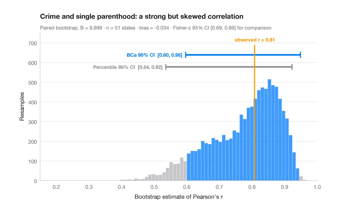
Bootstrap distribution
Resampled correlation with percentile and BCa 95% confidence intervals.
boot::boot() + boot::boot.ci()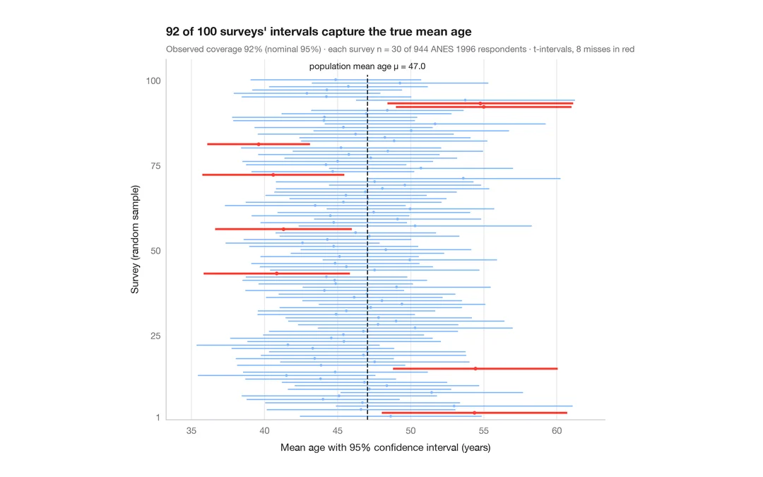
What a 95% confidence interval means
100 surveys of 30 people drawn from 944 ANES respondents; the 95% CIs for mean age that miss the true value are in red.
teaching classic (e.g. TeachingDemos::ci.examp())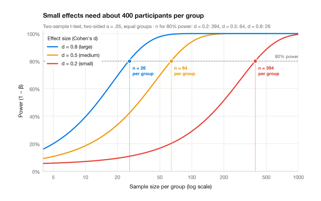
Power curve
Power of a two-sample t-test against sample size for small, medium and large effects.
pwr::pwr.t.test() + plot()