Funnel plot
Are small "Pygmalion" studies more optimistic? 19 teacher-expectancy effects against their standard error, with a pseudo 95% funnel and Egger's test.
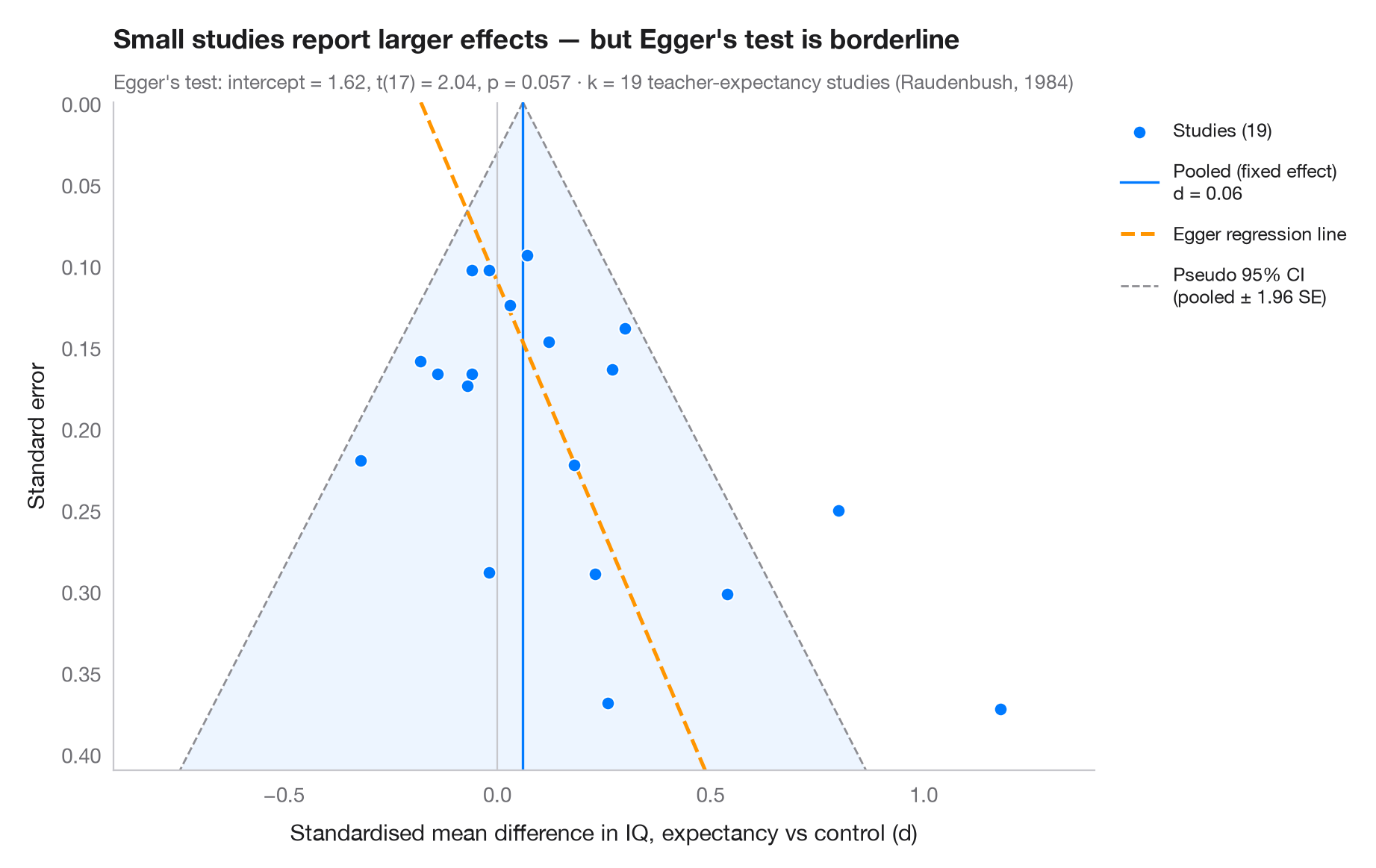
Each dot is a study: its effect size on the x-axis, its standard error on the (inverted) y-axis, so large precise studies sit at the top. Without bias the dots form a symmetric funnel around the pooled effect, 95% of them inside the pseudo-confidence region (± 1.96 SE). If small studies with null or negative results are missing — publication bias — the bottom of the funnel is lopsided. Egger's regression test (standard normal deviate on precision) quantifies that asymmetry; its fitted line is dashed.
Data are the 19 teacher-expectancy ("Pygmalion") experiments of Raudenbush
(1984): standardised mean differences in pupils' IQ and their sampling
variances, typed in as published in dat.raudenbush1985 of R's metafor.
The least precise studies report the largest effects, and Egger's intercept
is borderline. Asymmetry is not proof of publication bias: here the small
studies are mostly those in which teachers had known their pupils for a week
or less, which Raudenbush showed produces genuinely larger effects. Egger's
test is an OLS fit from statsmodels.
import matplotlib.pyplot as plt
import numpy as np
import statsmodels.api as sm

# Teacher-expectancy experiments (Raudenbush, 1984): standardised mean difference
# in pupil IQ and its sampling variance, as in metafor's dat.raudenbush1985
dp = np.array([0.03, 0.12, -0.14, 1.18, 0.26, -0.06, -0.02, -0.32, 0.27, 0.80, 0.54, 0.18,
               -0.02, 0.23, -0.18, -0.06, 0.30, 0.07, -0.07])
vi = np.array([0.0156, 0.0216, 0.0279, 0.1391, 0.1362, 0.0106, 0.0106, 0.0484, 0.0269, 0.0630,
               0.0912, 0.0497, 0.0835, 0.0841, 0.0253, 0.0279, 0.0193, 0.0088, 0.0303])
sp = np.sqrt(vi)

# Fixed-effect pooled estimate and Egger's test: z = b0 + b1 · precision
w = 1 / sp**2
pooled = np.sum(w * dp) / w.sum()
egger = sm.OLS(dp / sp, sm.add_constant(1 / sp)).fit()
b0, b1 = egger.params

fig, ax = plt.subplots(figsize=(9, 5.6))
s_grid = np.linspace(0, sp.max() * 1.1, 100)
ax.fill_betweenx(s_grid, pooled - 1.96 * s_grid, pooled + 1.96 * s_grid, color="#007AFF",
                 alpha=0.07, lw=0)
for sign in (-1, 1):
    ax.plot(pooled + sign * 1.96 * s_grid, s_grid, color="#8E8E93", lw=1, ls="--",
            label="Pseudo 95% CI\n(pooled ± 1.96 SE)" if sign > 0 else None)
ax.axvline(pooled, color="#007AFF", lw=1.2, label=f"Pooled (fixed effect)\nd = {pooled:.2f}")
ax.axvline(0, color="#C7C7CC", lw=0.8)
ax.plot(b1 + b0 * s_grid, s_grid, color="#FF9500", lw=1.8, ls="--", label="Egger regression line")

ax.scatter(dp, sp, s=40, color="#007AFF", edgecolor="white", lw=0.7, zorder=3,
           label=f"Studies ({len(dp)})")

ax.invert_yaxis()
ax.set_ylim(sp.max() * 1.1, 0)
ax.set_xlim(-0.9, 1.4)
ax.set_xlabel("Standardised mean difference in IQ, expectancy vs control (d)")
ax.set_ylabel("Standard error")
ax.grid(axis="y", visible=False)

handles, labels = ax.get_legend_handles_labels()
order = [3, 1, 2, 0]
ax.legend([handles[i] for i in order], [labels[i] for i in order], loc="upper left",
          bbox_to_anchor=(1.01, 1), fontsize=9, labelspacing=1)

ax.set_title("Small studies report larger effects — " + ("Egger's test flags asymmetry"
             if egger.pvalues[0] < 0.05 else "but Egger's test is borderline"), pad=26)
ax.text(0, 1.02, f"Egger's test: intercept = {b0:.2f}, t({egger.df_resid:.0f}) = "
        f"{egger.tvalues[0]:.2f}, p = {egger.pvalues[0]:.3f} · k = {len(dp)} teacher-expectancy "
        f"studies (Raudenbush, 1984)", transform=ax.transAxes, fontsize=9.5, color="#6E6E73")
plt.show()
Figures use the optional PyStatlas style: add plt.style.use("pystatlas.mplstyle") to match the look exactly.
Data source
- Teacher-expectancy experiments (Raudenbush, 1984). Raudenbush, S. W. (1984). Magnitude of teacher expectancy effects on pupil IQ as a function of the credibility of expectancy induction: A synthesis of findings from 18 experiments. Journal of Educational Psychology, 76(1), 85–97. https://doi.org/10.1037/0022-0663.76.1.85
Effect sizes and variances typed in from dat.raudenbush1985 in R's metadat/metafor (Viechtbauer, 2010, Journal of Statistical Software, 36(3), https://doi.org/10.18637/jss.v036.i03); one of the 18 experiments contributes two rows.
The examples illustrate statistical methods. Their titles describe what each figure shows in these particular data — often a small, dated or partial sample — not the author's position on the substantive question. For interpretation, context and data quality, rely on the original sources cited here.
How to cite
PyStatlas is created and maintained by Thierry Warin. If it helped your work, please cite it.
Warin, T. (2026). Funnel plot. In PyStatlas: A Python Gallery of Statistical Graphics for the Social Sciences. https://warint.github.io/pystatlas/inference-uncertainty/funnel-plot/
@misc{warin2026statlas,
  author       = {Warin, Thierry},
  title        = {PyStatlas: A Python Gallery of Statistical Graphics for the Social Sciences},
  year         = {2026},
  howpublished = {\url{https://warint.github.io/pystatlas/}},
  note         = {Source code: https://github.com/warint/pystatlas}
}More in Inference & uncertainty
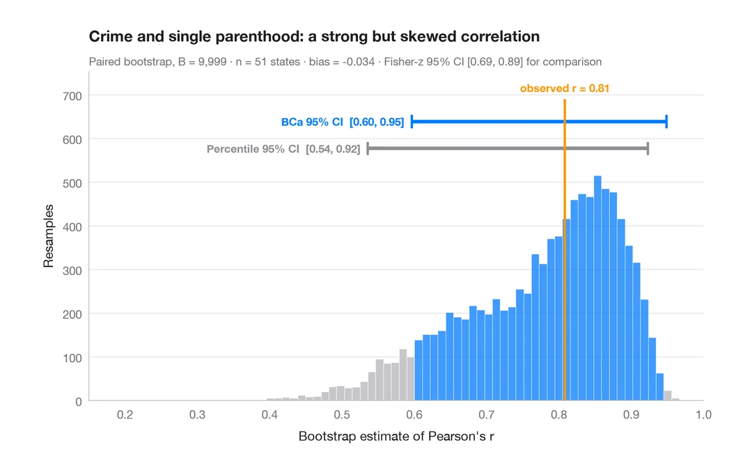
Bootstrap distribution
Resampled correlation with percentile and BCa 95% confidence intervals.
boot::boot() + boot::boot.ci()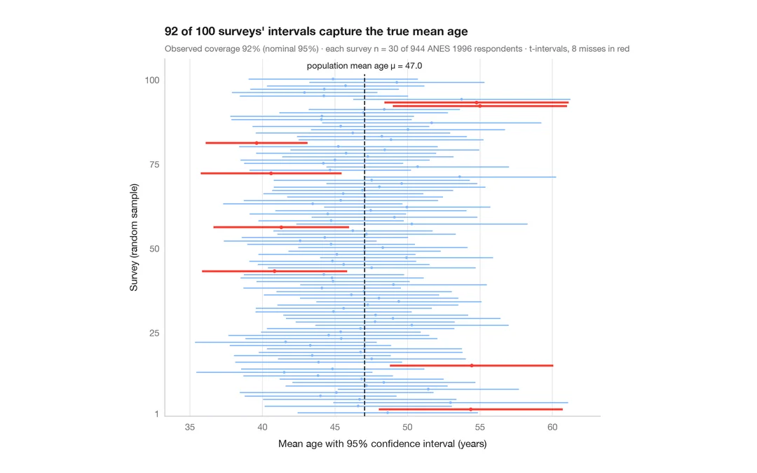
What a 95% confidence interval means
100 surveys of 30 people drawn from 944 ANES respondents; the 95% CIs for mean age that miss the true value are in red.
teaching classic (e.g. TeachingDemos::ci.examp())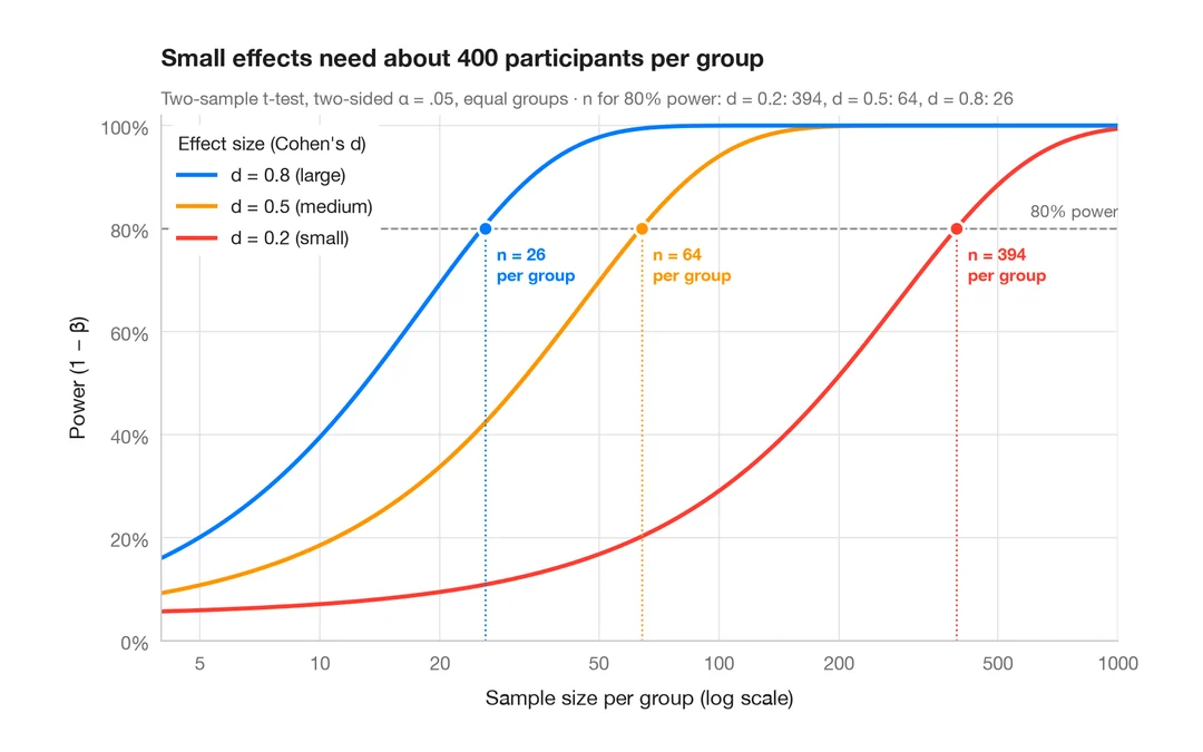
Power curve
Power of a two-sample t-test against sample size for small, medium and large effects.
pwr::pwr.t.test() + plot()