Funnel plot — PyStatlas: A Python Gallery of Statistical Graphics for the Social Sciences

Warin, Thierry

ファンネルプロット

小規模な「ピグマリオン」研究ほど楽観的か？教師期待の効果 19 件を標準誤差に対して描き、疑似 95% ファンネルと Egger 検定を添えます。

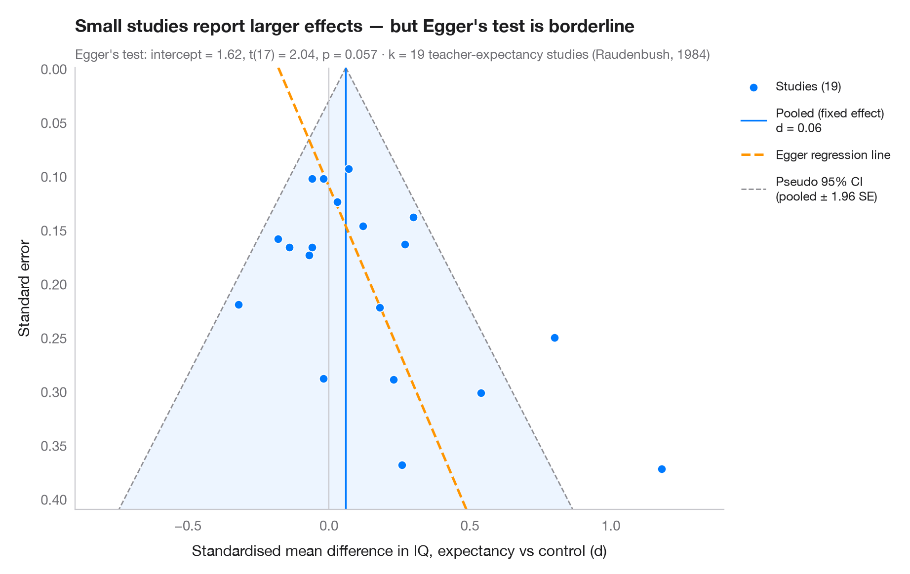
各点が 1 つの研究で、横軸に効果量、縦軸（反転）に標準誤差をとるため、大規模で精度の高い研究が上に来ます。バイアスがなければ、点は統合効果を中心とする対称なファンネルをなし、その 95% が疑似信頼領域（± 1.96 SE）に入ります。結果がゼロや負の小規模研究が欠けている — 出版バイアス — 場合、ファンネルの下部が偏ります。Egger の回帰検定（標準正規偏差を精度に回帰）がこの非対称性を定量化し、その当てはめ線を破線で示します。

データは Raudenbush (1984) の教師期待（「ピグマリオン」）実験 19 件で、児童の IQ の標準化平均差とその標本分散を、R の metafor の dat.raudenbush1985 に公表された値のまま入力しています。精度の低い研究ほど大きな効果を報告しており、Egger の切片は有意水準の境界付近です。非対称性は出版バイアスの証明ではありません。ここでは小規模研究の多くが、教師が児童を知って 1 週間以内の研究であり、Raudenbush はこの条件で実際に効果が大きくなることを示しました。Egger 検定は statsmodels の OLS によります。

コードおよび図中のテキストは英語です。

funnel-plot.py · 50 行

ダウンロード GitHub

import matplotlib.pyplot as plt
import numpy as np
import statsmodels.api as sm

# Teacher-expectancy experiments (Raudenbush, 1984): standardised mean difference
# in pupil IQ and its sampling variance, as in metafor's dat.raudenbush1985
dp = np.array([0.03, 0.12, -0.14, 1.18, 0.26, -0.06, -0.02, -0.32, 0.27, 0.80, 0.54, 0.18,
               -0.02, 0.23, -0.18, -0.06, 0.30, 0.07, -0.07])
vi = np.array([0.0156, 0.0216, 0.0279, 0.1391, 0.1362, 0.0106, 0.0106, 0.0484, 0.0269, 0.0630,
               0.0912, 0.0497, 0.0835, 0.0841, 0.0253, 0.0279, 0.0193, 0.0088, 0.0303])
sp = np.sqrt(vi)

# Fixed-effect pooled estimate and Egger's test: z = b0 + b1 · precision
w = 1 / sp**2
pooled = np.sum(w * dp) / w.sum()
egger = sm.OLS(dp / sp, sm.add_constant(1 / sp)).fit()
b0, b1 = egger.params

fig, ax = plt.subplots(figsize=(9, 5.6))
s_grid = np.linspace(0, sp.max() * 1.1, 100)
ax.fill_betweenx(s_grid, pooled - 1.96 * s_grid, pooled + 1.96 * s_grid, color="#007AFF",
                 alpha=0.07, lw=0)
for sign in (-1, 1):
    ax.plot(pooled + sign * 1.96 * s_grid, s_grid, color="#8E8E93", lw=1, ls="--",
            label="Pseudo 95% CI\n(pooled ± 1.96 SE)" if sign > 0 else None)
ax.axvline(pooled, color="#007AFF", lw=1.2, label=f"Pooled (fixed effect)\nd = {pooled:.2f}")
ax.axvline(0, color="#C7C7CC", lw=0.8)
ax.plot(b1 + b0 * s_grid, s_grid, color="#FF9500", lw=1.8, ls="--", label="Egger regression line")

ax.scatter(dp, sp, s=40, color="#007AFF", edgecolor="white", lw=0.7, zorder=3,
           label=f"Studies ({len(dp)})")

ax.invert_yaxis()
ax.set_ylim(sp.max() * 1.1, 0)
ax.set_xlim(-0.9, 1.4)
ax.set_xlabel("Standardised mean difference in IQ, expectancy vs control (d)")
ax.set_ylabel("Standard error")
ax.grid(axis="y", visible=False)

handles, labels = ax.get_legend_handles_labels()
order = [3, 1, 2, 0]
ax.legend([handles[i] for i in order], [labels[i] for i in order], loc="upper left",
          bbox_to_anchor=(1.01, 1), fontsize=9, labelspacing=1)

ax.set_title("Small studies report larger effects — " + ("Egger's test flags asymmetry"
             if egger.pvalues[0] < 0.05 else "but Egger's test is borderline"), pad=26)
ax.text(0, 1.02, f"Egger's test: intercept = {b0:.2f}, t({egger.df_resid:.0f}) = "
        f"{egger.tvalues[0]:.2f}, p = {egger.pvalues[0]:.3f} · k = {len(dp)} teacher-expectancy "
        f"studies (Raudenbush, 1984)", transform=ax.transAxes, fontsize=9.5, color="#6E6E73")
plt.show()

図にはオプションの PyStatlas スタイルを使用しています。同じ見た目にするには plt.style.use("pystatlas.mplstyle") を追加してください。

データの出典

Teacher-expectancy experiments (Raudenbush, 1984). Raudenbush, S. W. (1984). Magnitude of teacher expectancy effects on pupil IQ as a function of the credibility of expectancy induction: A synthesis of findings from 18 experiments. Journal of Educational Psychology, 76(1), 85–97. https://doi.org/10.1037/0022-0663.76.1.85
Effect sizes and variances typed in from dat.raudenbush1985 in R's metadat/metafor (Viechtbauer, 2010, Journal of Statistical Software, 36(3), https://doi.org/10.18637/jss.v036.i03); one of the 18 experiments contributes two rows.

これらの例は統計手法を説明するためのものです。図のタイトルは、この特定のデータ（多くは小規模で、古く、部分的な標本）で図が示す内容を述べたものであり、実質的な問いに対する著者の立場ではありません。解釈、背景、データの質については、ここに挙げた元の出典を参照してください。

引用方法

PyStatlas は Thierry Warin が作成・運営しています。研究や業務に役立った場合は、ぜひ引用してください。

Warin, T. (2026). Funnel plot. In PyStatlas: A Python Gallery of Statistical Graphics for the Social Sciences. https://warint.github.io/pystatlas/inference-uncertainty/funnel-plot/

@misc{warin2026statlas,
  author       = {Warin, Thierry},
  title        = {PyStatlas: A Python Gallery of Statistical Graphics for the Social Sciences},
  year         = {2026},
  howpublished = {\url{https://warint.github.io/pystatlas/}},
  note         = {Source code: https://github.com/warint/pystatlas}
}

推測と不確実性のその他のグラフ

推測と不確実性

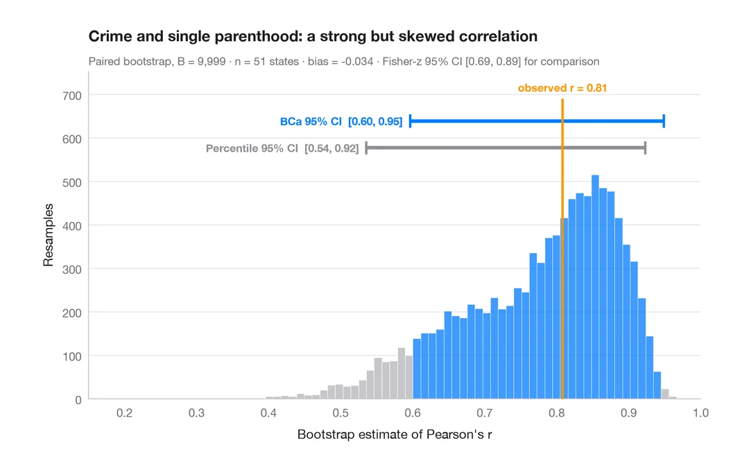
ブートストラップ分布

再標本化した相関係数を、パーセンタイル法と BCa 法の 95% 信頼区間とともに示します。

boot::boot() + boot::boot.ci()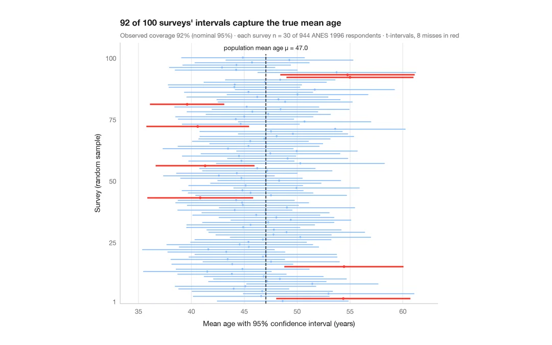

推測と不確実性

95% 信頼区間の意味

ANES の回答者 944 人から 30 人を抽出する調査を 100 回。平均年齢の 95% 信頼区間のうち真値を外したものを赤で示します。

teaching classic (e.g. TeachingDemos::ci.examp())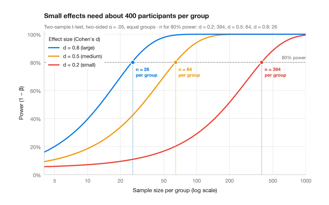

推測と不確実性

検出力曲線

2標本 t 検定の検出力を、小・中・大の効果量ごとに標本サイズに対して描きます。

pwr::pwr.t.test() + plot()