ブートストラップ分布
再標本化した相関係数を、パーセンタイル法と BCa 法の 95% 信頼区間とともに示します。
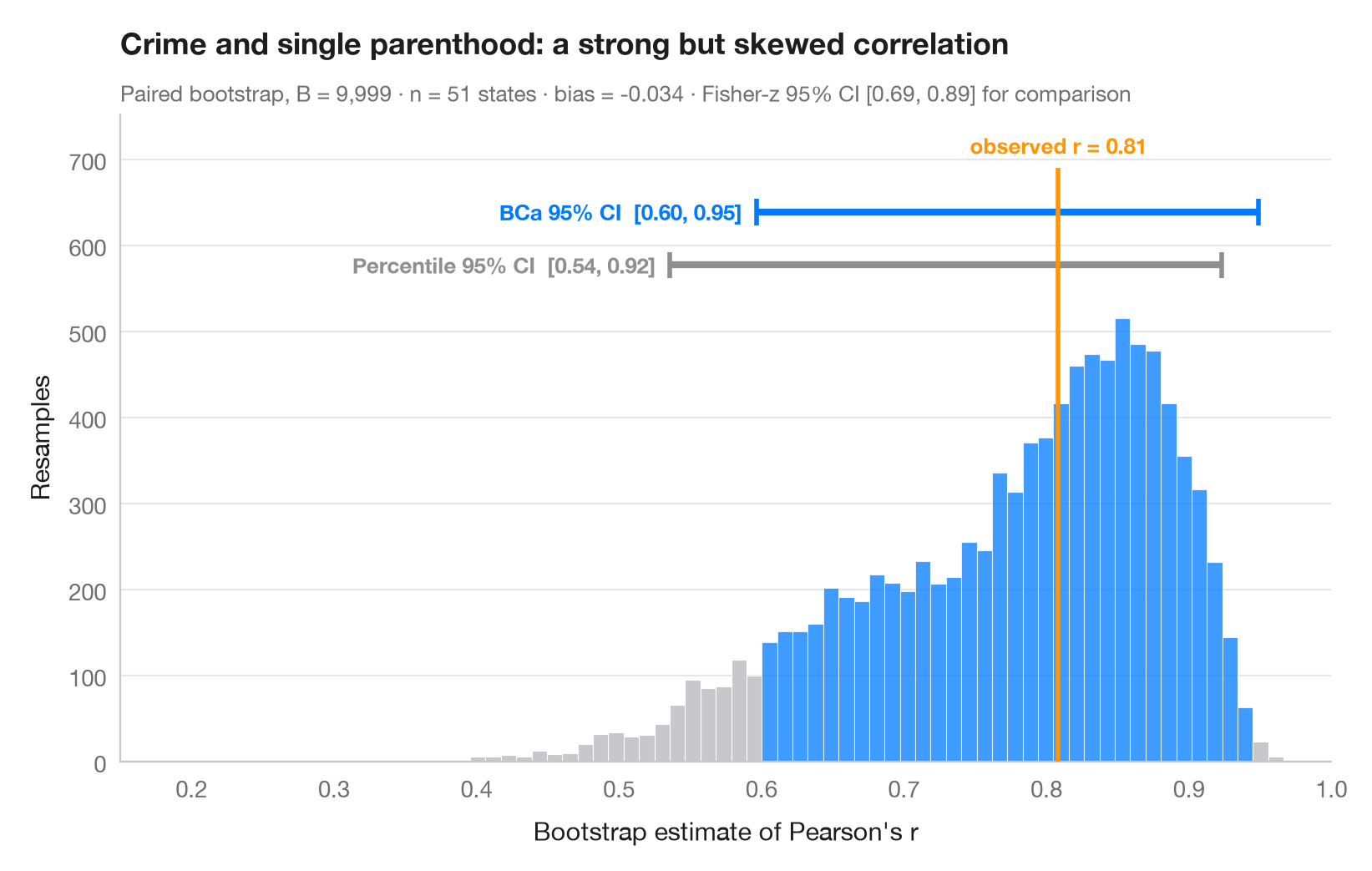
ブートストラップは、データから復元抽出した何千もの標本で統計量を推定し直します。その推定値のばらつきが標本抽出に伴う不確実性です。ヒストグラムは相関係数のブートストラップ分布、オレンジの線は全標本で観測された値です。その上に2つの 95% 区間を描いています。単純な パーセンタイル 区間と、BCa(バイアス補正・加速)区間です。後者はここに見られる偏りと歪みを考慮してずれており、分布は対称からほど遠いことがわかります。
データは statsmodels の statecrime データセットに含まれる米国50州+DC で、ひとり親世帯の割合と凶悪犯罪率を対比しています。両方の区間は scipy.stats.bootstrap(対応あり、9,999 回の再標本化)で求めています。
コードおよび図中のテキストは英語です。
import matplotlib.pyplot as plt
import numpy as np
import statsmodels.api as sm
from scipy import stats

# Data: violent crime vs single-parent households, 51 states
df = sm.datasets.statecrime.load_pandas().data
x, y = df["single"].to_numpy(), df["violent"].to_numpy()
r_obs = stats.pearsonr(x, y)[0]

# Paired bootstrap of Pearson's r: percentile and BCa intervals from the same resamples
r = lambda a, b, axis=-1: stats.pearsonr(a, b, axis=axis)[0]
boot = {m: stats.bootstrap((x, y), r, paired=True, vectorized=True, n_resamples=9999,
                           method=m, random_state=np.random.default_rng(7))
        for m in ["percentile", "BCa"]}
dist = boot["BCa"].bootstrap_distribution
fisher = np.tanh(np.arctanh(r_obs) + np.array([-1, 1]) * 1.96 / np.sqrt(len(x) - 3))

fig, ax = plt.subplots(figsize=(8, 5))
lo, hi = boot["BCa"].confidence_interval
counts, edges, bars = ax.hist(dist, bins=60, color="#C7C7CC", edgecolor="white", lw=0.4)
for b, left in zip(bars, edges[:-1]):
    if lo <= left + (edges[1] - edges[0]) / 2 <= hi:
        b.set_facecolor("#007AFF"); b.set_alpha(0.75)

# Intervals stacked above the histogram
top = counts.max()
for i, (m, c, name) in enumerate([("percentile", "#8E8E93", "Percentile"),
                                  ("BCa", "#007AFF", "BCa")]):
    a, b = boot[m].confidence_interval
    yy = top * (1.12 + 0.12 * i)
    ax.plot([a, b], [yy, yy], color=c, lw=3, solid_capstyle="butt")
    ax.vlines([a, b], yy - top * 0.03, yy + top * 0.03, color=c, lw=2)
    ax.text(a - 0.01, yy, f"{name} 95% CI  [{a:.2f}, {b:.2f}]", ha="right", va="center",
            fontsize=9.5, color=c, fontweight="semibold")

ax.vlines(r_obs, 0, top * 1.34, color="#FF9500", lw=2, zorder=3)
ax.text(r_obs, top * 1.36, f"observed r = {r_obs:.2f}", ha="center", va="bottom",
        fontsize=9.5, color="#FF9500", fontweight="semibold")
ax.set_xlim(0.15, 1)
ax.set_ylim(0, top * 1.46)
ax.set_xlabel("Bootstrap estimate of Pearson's r")
ax.set_ylabel("Resamples")
ax.set_title("Crime and single parenthood: a strong but skewed correlation", pad=26)
ax.text(0, 1.02, f"Paired bootstrap, B = 9,999 · n = {len(x)} states · bias = "
        f"{dist.mean() - r_obs:+.3f} · Fisher-z 95% CI [{fisher[0]:.2f}, {fisher[1]:.2f}] for comparison",
        transform=ax.transAxes, fontsize=9.5, color="#6E6E73")
plt.show()
図にはオプションの PyStatlas スタイル を使用しています。同じ見た目にするには plt.style.use("pystatlas.mplstyle") を追加してください。
データの出典
- US state crime and social indicators, 2009. U.S. Census Bureau. Statistical Abstract of the United States, state tables for 2009 (crime rates from the FBI Uniform Crime Reporting program). https://www.statsmodels.org/stable/datasets/generated/statecrime.html
Compiled for statsmodels (sm.datasets.statecrime); public domain. See the statsmodels page for each variable's table and footnotes.
これらの例は統計手法を説明するためのものです。図のタイトルは、この特定のデータ(多くは小規模で、古く、部分的な標本)で図が示す内容を述べたものであり、実質的な問いに対する著者の立場ではありません。解釈、背景、データの質については、ここに挙げた元の出典を参照してください。
引用方法
PyStatlas は Thierry Warin が作成・運営しています。研究や業務に役立った場合は、ぜひ引用してください。
Warin, T. (2026). Bootstrap distribution. In PyStatlas: A Python Gallery of Statistical Graphics for the Social Sciences. https://warint.github.io/pystatlas/inference-uncertainty/bootstrap-distribution/
@misc{warin2026statlas,
  author       = {Warin, Thierry},
  title        = {PyStatlas: A Python Gallery of Statistical Graphics for the Social Sciences},
  year         = {2026},
  howpublished = {\url{https://warint.github.io/pystatlas/}},
  note         = {Source code: https://github.com/warint/pystatlas}
}推測と不確実性のその他のグラフ
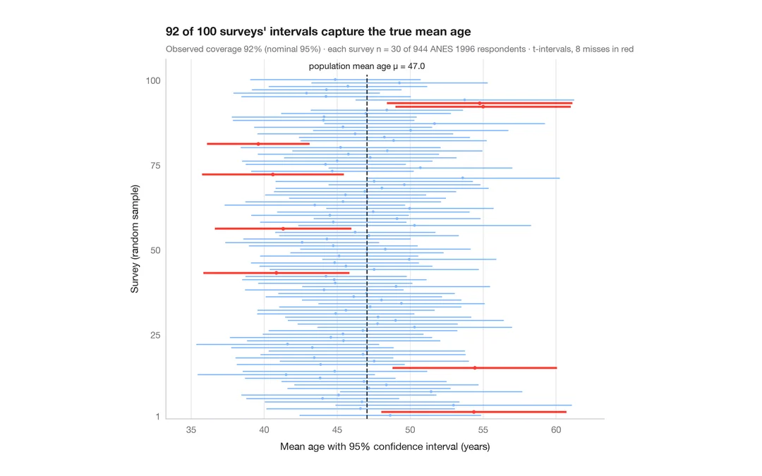
95% 信頼区間の意味
ANES の回答者 944 人から 30 人を抽出する調査を 100 回。平均年齢の 95% 信頼区間のうち真値を外したものを赤で示します。
teaching classic (e.g. TeachingDemos::ci.examp())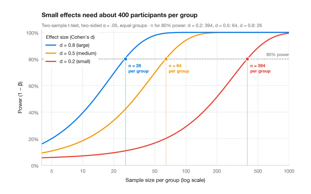
検出力曲線
2標本 t 検定の検出力を、小・中・大の効果量ごとに標本サイズに対して描きます。
pwr::pwr.t.test() + plot()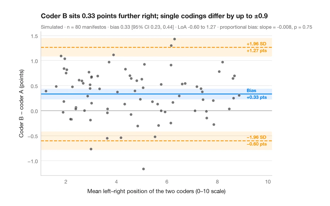
ブランド・アルトマンプロット
2 人のコーダーは政党の選挙綱領を左右軸上に同じように位置づけるか?バイアスと 95% 一致限界。
BlandAltmanLeh::bland.altman.plot() / blandr::blandr.draw()