Distribution bootstrap
Corrélation rééchantillonnée avec intervalles de confiance à 95 % par percentiles et BCa.
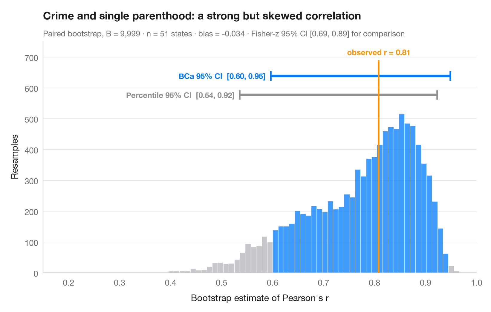
Le bootstrap réestime une statistique sur des milliers d'échantillons tirés avec remise dans les données ; la dispersion de ces estimations mesure son incertitude d'échantillonnage. L'histogramme est la distribution bootstrap d'une corrélation, la ligne orange la valeur observée dans l'échantillon complet. Deux intervalles à 95 % sont tracés au-dessus : l'intervalle simple par percentiles et l'intervalle BCa (corrigé du biais et accéléré), qui se déplace pour tenir compte du biais et de l'asymétrie visibles ici — la distribution est loin d'être symétrique.
Les données sont les 50 États américains + DC du jeu de données statecrime de statsmodels : la proportion de familles monoparentales en regard du taux de crimes violents. scipy.stats.bootstrap (apparié, 9 999 rééchantillonnages) fournit les deux intervalles.
Le code et le texte à l'intérieur des figures sont en anglais.
import matplotlib.pyplot as plt
import numpy as np
import statsmodels.api as sm
from scipy import stats

# Data: violent crime vs single-parent households, 51 states
df = sm.datasets.statecrime.load_pandas().data
x, y = df["single"].to_numpy(), df["violent"].to_numpy()
r_obs = stats.pearsonr(x, y)[0]

# Paired bootstrap of Pearson's r: percentile and BCa intervals from the same resamples
r = lambda a, b, axis=-1: stats.pearsonr(a, b, axis=axis)[0]
boot = {m: stats.bootstrap((x, y), r, paired=True, vectorized=True, n_resamples=9999,
                           method=m, random_state=np.random.default_rng(7))
        for m in ["percentile", "BCa"]}
dist = boot["BCa"].bootstrap_distribution
fisher = np.tanh(np.arctanh(r_obs) + np.array([-1, 1]) * 1.96 / np.sqrt(len(x) - 3))

fig, ax = plt.subplots(figsize=(8, 5))
lo, hi = boot["BCa"].confidence_interval
counts, edges, bars = ax.hist(dist, bins=60, color="#C7C7CC", edgecolor="white", lw=0.4)
for b, left in zip(bars, edges[:-1]):
    if lo <= left + (edges[1] - edges[0]) / 2 <= hi:
        b.set_facecolor("#007AFF"); b.set_alpha(0.75)

# Intervals stacked above the histogram
top = counts.max()
for i, (m, c, name) in enumerate([("percentile", "#8E8E93", "Percentile"),
                                  ("BCa", "#007AFF", "BCa")]):
    a, b = boot[m].confidence_interval
    yy = top * (1.12 + 0.12 * i)
    ax.plot([a, b], [yy, yy], color=c, lw=3, solid_capstyle="butt")
    ax.vlines([a, b], yy - top * 0.03, yy + top * 0.03, color=c, lw=2)
    ax.text(a - 0.01, yy, f"{name} 95% CI  [{a:.2f}, {b:.2f}]", ha="right", va="center",
            fontsize=9.5, color=c, fontweight="semibold")

ax.vlines(r_obs, 0, top * 1.34, color="#FF9500", lw=2, zorder=3)
ax.text(r_obs, top * 1.36, f"observed r = {r_obs:.2f}", ha="center", va="bottom",
        fontsize=9.5, color="#FF9500", fontweight="semibold")
ax.set_xlim(0.15, 1)
ax.set_ylim(0, top * 1.46)
ax.set_xlabel("Bootstrap estimate of Pearson's r")
ax.set_ylabel("Resamples")
ax.set_title("Crime and single parenthood: a strong but skewed correlation", pad=26)
ax.text(0, 1.02, f"Paired bootstrap, B = 9,999 · n = {len(x)} states · bias = "
        f"{dist.mean() - r_obs:+.3f} · Fisher-z 95% CI [{fisher[0]:.2f}, {fisher[1]:.2f}] for comparison",
        transform=ax.transAxes, fontsize=9.5, color="#6E6E73")
plt.show()
Les figures utilisent le style PyStatlas (facultatif) : ajoutez plt.style.use("pystatlas.mplstyle") pour obtenir exactement le même rendu.
Source des données
- US state crime and social indicators, 2009. U.S. Census Bureau. Statistical Abstract of the United States, state tables for 2009 (crime rates from the FBI Uniform Crime Reporting program). https://www.statsmodels.org/stable/datasets/generated/statecrime.html
Compiled for statsmodels (sm.datasets.statecrime); public domain. See the statsmodels page for each variable's table and footnotes.
Les exemples illustrent des méthodes statistiques. Leurs titres décrivent ce que chaque figure montre dans ces données précises — souvent un échantillon restreint, daté ou partiel —, et non la position de l'auteur sur la question de fond. Pour l'interprétation, le contexte et la qualité des données, reportez-vous aux sources originales citées ici.
Comment citer
PyStatlas est créé et maintenu par Thierry Warin. S'il vous a été utile dans vos travaux, merci de le citer.
Warin, T. (2026). Bootstrap distribution. In PyStatlas: A Python Gallery of Statistical Graphics for the Social Sciences. https://warint.github.io/pystatlas/inference-uncertainty/bootstrap-distribution/
@misc{warin2026statlas,
  author       = {Warin, Thierry},
  title        = {PyStatlas: A Python Gallery of Statistical Graphics for the Social Sciences},
  year         = {2026},
  howpublished = {\url{https://warint.github.io/pystatlas/}},
  note         = {Source code: https://github.com/warint/pystatlas}
}Plus dans Inférence et incertitude
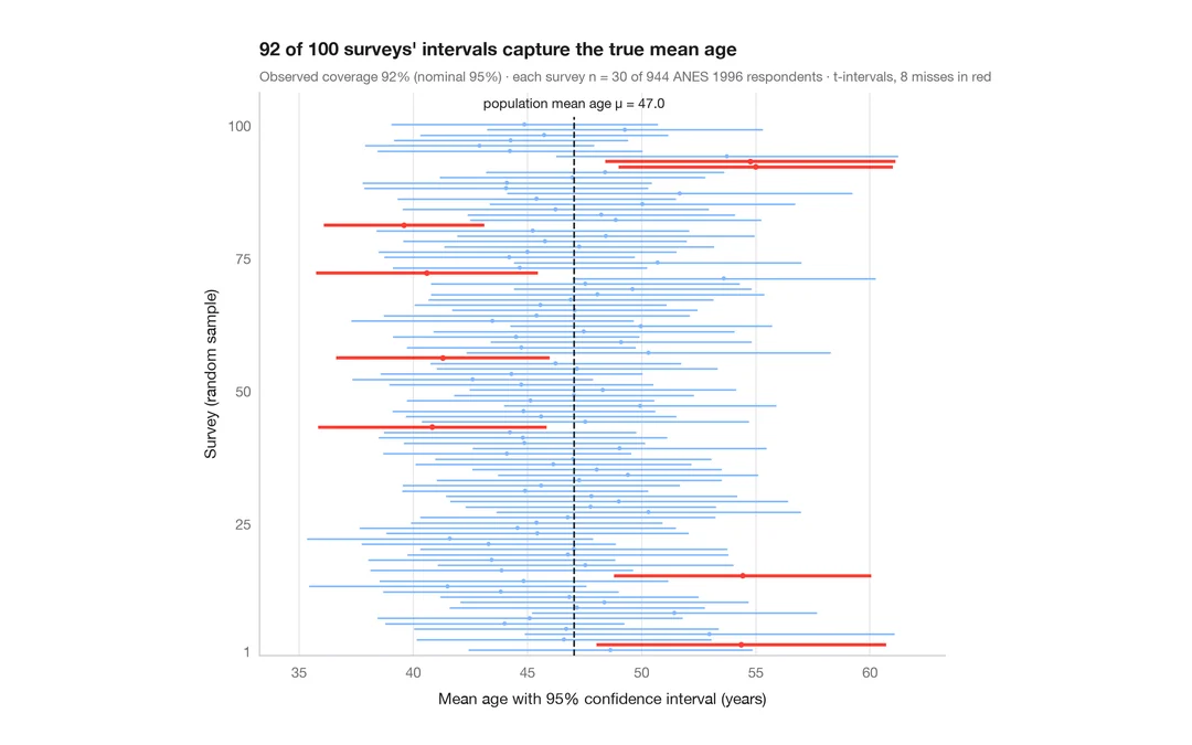
Ce que signifie un intervalle de confiance à 95 %
100 enquêtes de 30 personnes tirées parmi 944 répondants de l'ANES ; les IC à 95 % de l'âge moyen qui manquent la vraie valeur sont en rouge.
teaching classic (e.g. TeachingDemos::ci.examp())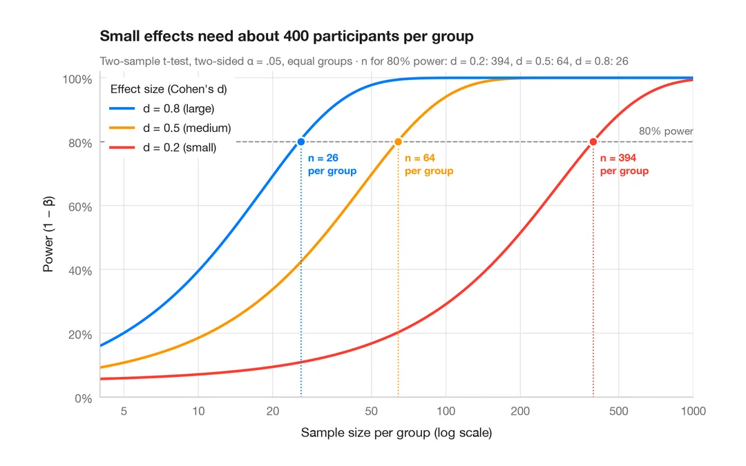
Courbe de puissance
Puissance d'un test t à deux échantillons selon la taille d'échantillon, pour des effets petits, moyens et grands.
pwr::pwr.t.test() + plot()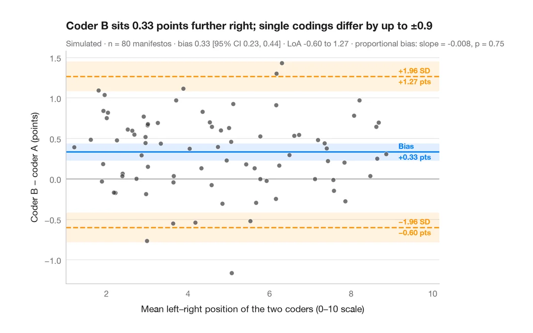
Graphique de Bland–Altman
Deux codeurs placent-ils les programmes électoraux de la même façon sur l'axe gauche–droite ? Biais et limites d'agrément à 95 %.
BlandAltmanLeh::bland.altman.plot() / blandr::blandr.draw()