Courbe de puissance
Puissance d'un test t à deux échantillons selon la taille d'échantillon, pour des effets petits, moyens et grands.
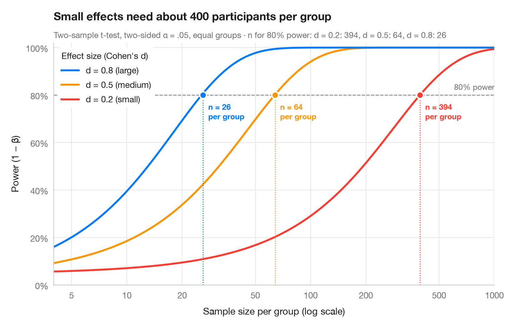
La puissance statistique est la probabilité qu'une étude détecte un effet qui existe réellement. Chaque courbe montre comment la puissance croît avec le nombre de participants par groupe, pour l'une des tailles d'effet de référence de Cohen (petite d = 0.2, moyenne 0.5, grande 0.8). Là où une courbe franchit la ligne conventionnelle des 80 %, un point indique la taille d'échantillon requise — remarquez à quelle vitesse elle explose lorsque l'effet diminue (l'axe des x est logarithmique).
Calculé avec statsmodels.stats.power.TTestIndPower : .power() pour les courbes et .solve_power() pour le n requis (α bilatéral = .05, groupes de tailles égales).
Le code et le texte à l'intérieur des figures sont en anglais.
import matplotlib.pyplot as plt
import numpy as np
from matplotlib.ticker import FixedLocator, NullLocator
from statsmodels.stats.power import TTestIndPower

analysis = TTestIndPower()
n = np.geomspace(4, 1000, 300)  # participants per group
effects = {0.2: ("small", "#FF3B30"), 0.5: ("medium", "#FF9500"), 0.8: ("large", "#007AFF")}

fig, ax = plt.subplots(figsize=(8, 5))
ax.axhline(0.8, color="#8E8E93", ls="--", lw=1)
ax.text(1000, 0.815, "80% power", ha="right", va="bottom", fontsize=9, color="#6E6E73")

required = {}
for d, (name, c) in effects.items():
    power = analysis.power(effect_size=d, nobs1=n, alpha=0.05)
    power = np.nan_to_num(power, nan=1.0)  # the noncentral t returns NaN once power ≈ 1
    ax.plot(n, power, color=c, lw=2.2,
            label=f"d = {d} ({name})")
    # Sample size per group that reaches 80% power
    n80 = int(np.ceil(analysis.solve_power(effect_size=d, power=0.8, alpha=0.05)))
    required[d] = n80
    ax.vlines(n80, 0, 0.8, color=c, lw=1, ls=":")
    ax.scatter(n80, 0.8, s=60, color=c, edgecolor="white", lw=1.5, zorder=4)
    ax.annotate(f"n = {n80}\nper group", (n80, 0.8), xytext=(6, -8), textcoords="offset points",
                ha="left", va="top", fontsize=9, color=c, fontweight="semibold")

handles, labels = ax.get_legend_handles_labels()
ax.legend(handles[::-1], labels[::-1], loc="upper left", title="Effect size (Cohen's d)",
          alignment="left", frameon=True, facecolor="white", edgecolor="none", framealpha=1)
ax.set_xscale("log")
ax.xaxis.set_major_locator(FixedLocator([5, 10, 20, 50, 100, 200, 500, 1000]))
ax.xaxis.set_minor_locator(NullLocator())
ax.xaxis.set_major_formatter(lambda v, _: f"{v:g}")
ax.set_xlim(4, 1000)
ax.set_ylim(0, 1.02)
ax.yaxis.set_major_formatter(lambda v, _: f"{v:.0%}")
ax.grid(axis="x")
ax.set_xlabel("Sample size per group (log scale)")
ax.set_ylabel("Power (1 − β)")
ax.set_title("Small effects need about 400 participants per group", pad=26)
ax.text(0, 1.02, "Two-sample t-test, two-sided α = .05, equal groups · n for 80% power: "
        + ", ".join(f"d = {d}: {k}" for d, k in required.items()),
        transform=ax.transAxes, fontsize=9.5, color="#6E6E73")
plt.show()
Les figures utilisent le style PyStatlas (facultatif) : ajoutez plt.style.use("pystatlas.mplstyle") pour obtenir exactement le même rendu.
Comment citer
PyStatlas est créé et maintenu par Thierry Warin. S'il vous a été utile dans vos travaux, merci de le citer.
Warin, T. (2026). Power curve. In PyStatlas: A Python Gallery of Statistical Graphics for the Social Sciences. https://warint.github.io/pystatlas/inference-uncertainty/power-curve/
@misc{warin2026statlas,
  author       = {Warin, Thierry},
  title        = {PyStatlas: A Python Gallery of Statistical Graphics for the Social Sciences},
  year         = {2026},
  howpublished = {\url{https://warint.github.io/pystatlas/}},
  note         = {Source code: https://github.com/warint/pystatlas}
}Plus dans Inférence et incertitude
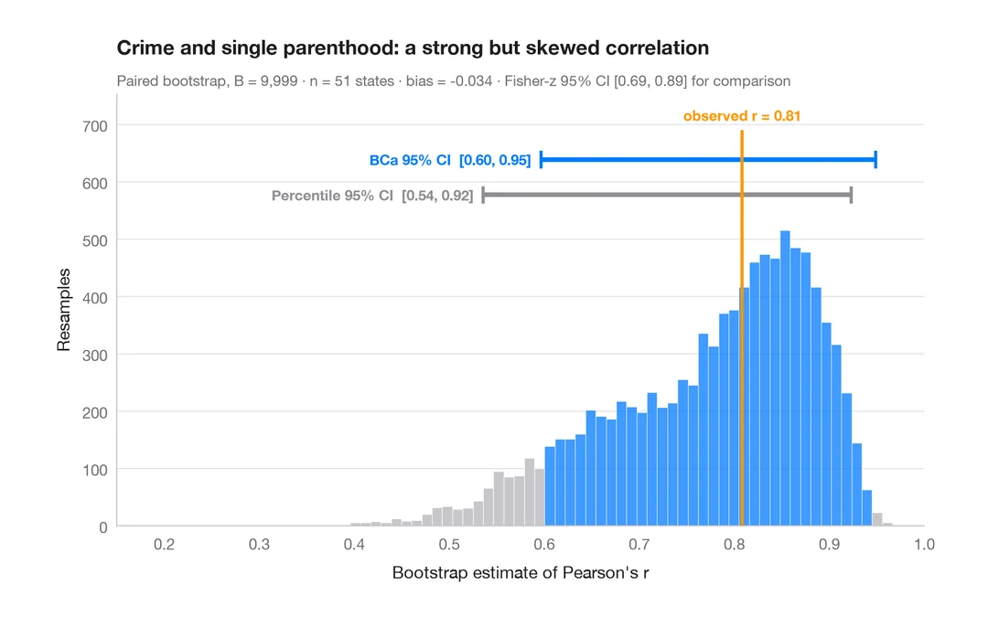
Distribution bootstrap
Corrélation rééchantillonnée avec intervalles de confiance à 95 % par percentiles et BCa.
boot::boot() + boot::boot.ci()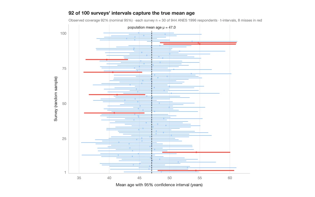
Ce que signifie un intervalle de confiance à 95 %
100 enquêtes de 30 personnes tirées parmi 944 répondants de l'ANES ; les IC à 95 % de l'âge moyen qui manquent la vraie valeur sont en rouge.
teaching classic (e.g. TeachingDemos::ci.examp())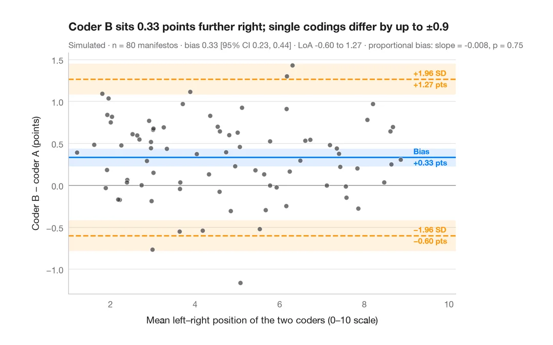
Graphique de Bland–Altman
Deux codeurs placent-ils les programmes électoraux de la même façon sur l'axe gauche–droite ? Biais et limites d'agrément à 95 %.
BlandAltmanLeh::bland.altman.plot() / blandr::blandr.draw()