Power curve

Warin, Thierry

Power of a two-sample t-test against sample size for small, medium and large effects.

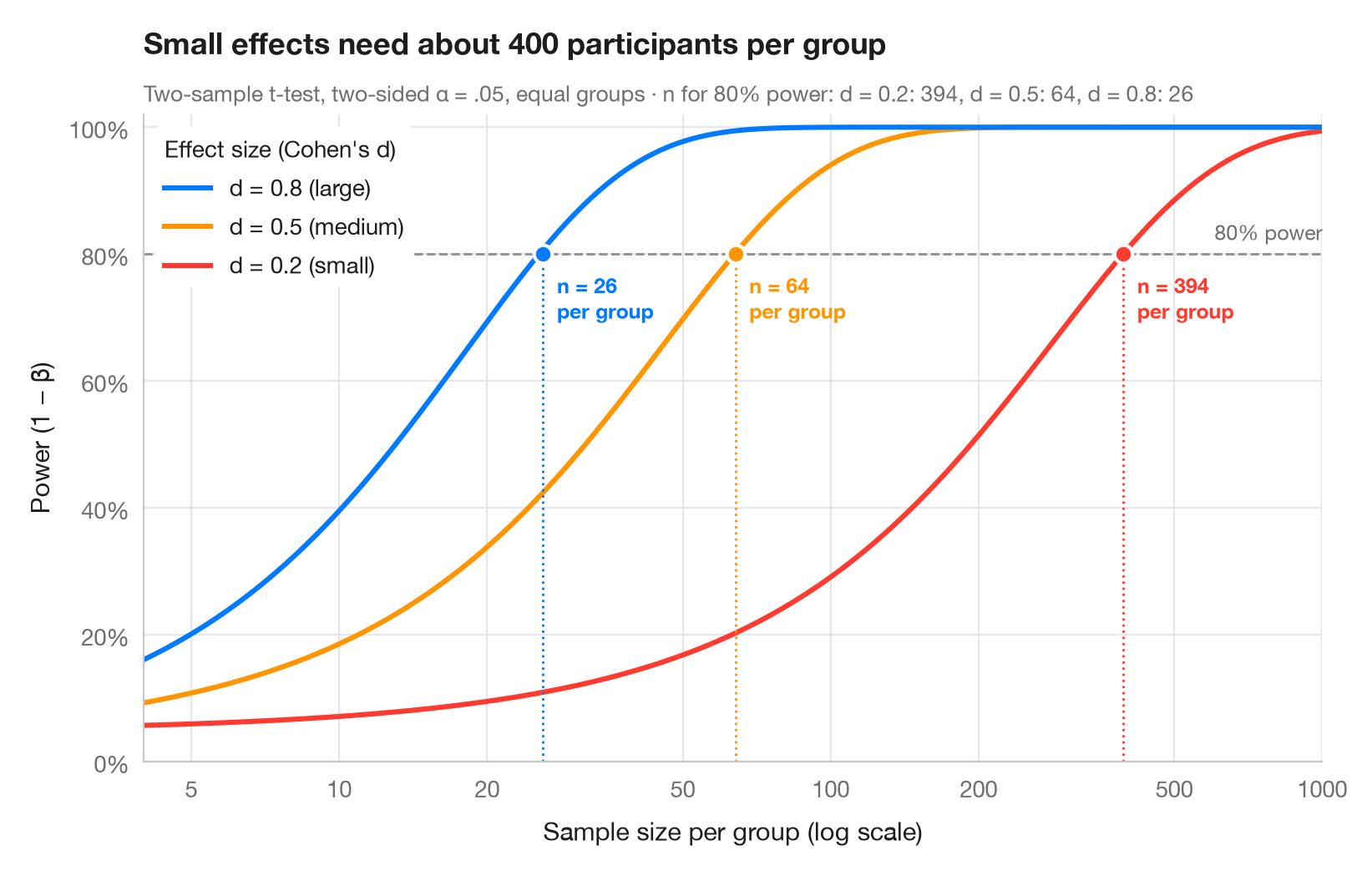
Statistical power is the probability that a study detects an effect that is really there. Each curve shows how power grows with the number of participants per group, for one of Cohen's benchmark effect sizes (small d = 0.2, medium 0.5, large 0.8). Where a curve crosses the conventional 80% line, a dot marks the sample size needed — note how quickly it explodes as the effect shrinks (the x-axis is logarithmic).

Computed with statsmodels.stats.power.TTestIndPower: .power() for the curves and .solve_power() for the required n (two-sided α = .05, equal group sizes).

power-curve.py · 45 lines

Download GitHub

import matplotlib.pyplot as plt
import numpy as np
from matplotlib.ticker import FixedLocator, NullLocator
from statsmodels.stats.power import TTestIndPower

analysis = TTestIndPower()
n = np.geomspace(4, 1000, 300)  # participants per group
effects = {0.2: ("small", "#FF3B30"), 0.5: ("medium", "#FF9500"), 0.8: ("large", "#007AFF")}

fig, ax = plt.subplots(figsize=(8, 5))
ax.axhline(0.8, color="#8E8E93", ls="--", lw=1)
ax.text(1000, 0.815, "80% power", ha="right", va="bottom", fontsize=9, color="#6E6E73")

required = {}
for d, (name, c) in effects.items():
    power = analysis.power(effect_size=d, nobs1=n, alpha=0.05)
    power = np.nan_to_num(power, nan=1.0)  # the noncentral t returns NaN once power ≈ 1
    ax.plot(n, power, color=c, lw=2.2,
            label=f"d = {d} ({name})")
    # Sample size per group that reaches 80% power
    n80 = int(np.ceil(analysis.solve_power(effect_size=d, power=0.8, alpha=0.05)))
    required[d] = n80
    ax.vlines(n80, 0, 0.8, color=c, lw=1, ls=":")
    ax.scatter(n80, 0.8, s=60, color=c, edgecolor="white", lw=1.5, zorder=4)
    ax.annotate(f"n = {n80}\nper group", (n80, 0.8), xytext=(6, -8), textcoords="offset points",
                ha="left", va="top", fontsize=9, color=c, fontweight="semibold")

handles, labels = ax.get_legend_handles_labels()
ax.legend(handles[::-1], labels[::-1], loc="upper left", title="Effect size (Cohen's d)",
          alignment="left", frameon=True, facecolor="white", edgecolor="none", framealpha=1)
ax.set_xscale("log")
ax.xaxis.set_major_locator(FixedLocator([5, 10, 20, 50, 100, 200, 500, 1000]))
ax.xaxis.set_minor_locator(NullLocator())
ax.xaxis.set_major_formatter(lambda v, _: f"{v:g}")
ax.set_xlim(4, 1000)
ax.set_ylim(0, 1.02)
ax.yaxis.set_major_formatter(lambda v, _: f"{v:.0%}")
ax.grid(axis="x")
ax.set_xlabel("Sample size per group (log scale)")
ax.set_ylabel("Power (1 − β)")
ax.set_title("Small effects need about 400 participants per group", pad=26)
ax.text(0, 1.02, "Two-sample t-test, two-sided α = .05, equal groups · n for 80% power: "
        + ", ".join(f"d = {d}: {k}" for d, k in required.items()),
        transform=ax.transAxes, fontsize=9.5, color="#6E6E73")
plt.show()

Figures use the optional PyStatlas style: add plt.style.use("pystatlas.mplstyle") to match the look exactly.

How to cite

PyStatlas is created and maintained by Thierry Warin. If it helped your work, please cite it.

Warin, T. (2026). Power curve. In PyStatlas: A Python Gallery of Statistical Graphics for the Social Sciences. https://warint.github.io/pystatlas/inference-uncertainty/power-curve/

@misc{warin2026statlas,
  author       = {Warin, Thierry},
  title        = {PyStatlas: A Python Gallery of Statistical Graphics for the Social Sciences},
  year         = {2026},
  howpublished = {\url{https://warint.github.io/pystatlas/}},
  note         = {Source code: https://github.com/warint/pystatlas}
}

More in Inference & uncertainty

Inference & uncertainty

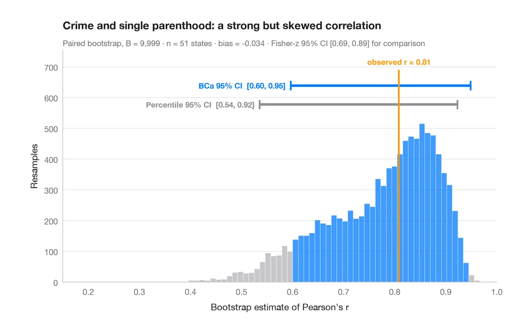
Bootstrap distribution

Resampled correlation with percentile and BCa 95% confidence intervals.

boot::boot() + boot::boot.ci()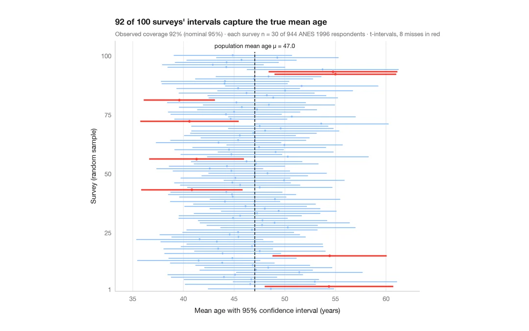

Inference & uncertainty

What a 95% confidence interval means

100 surveys of 30 people drawn from 944 ANES respondents; the 95% CIs for mean age that miss the true value are in red.

teaching classic (e.g. TeachingDemos::ci.examp())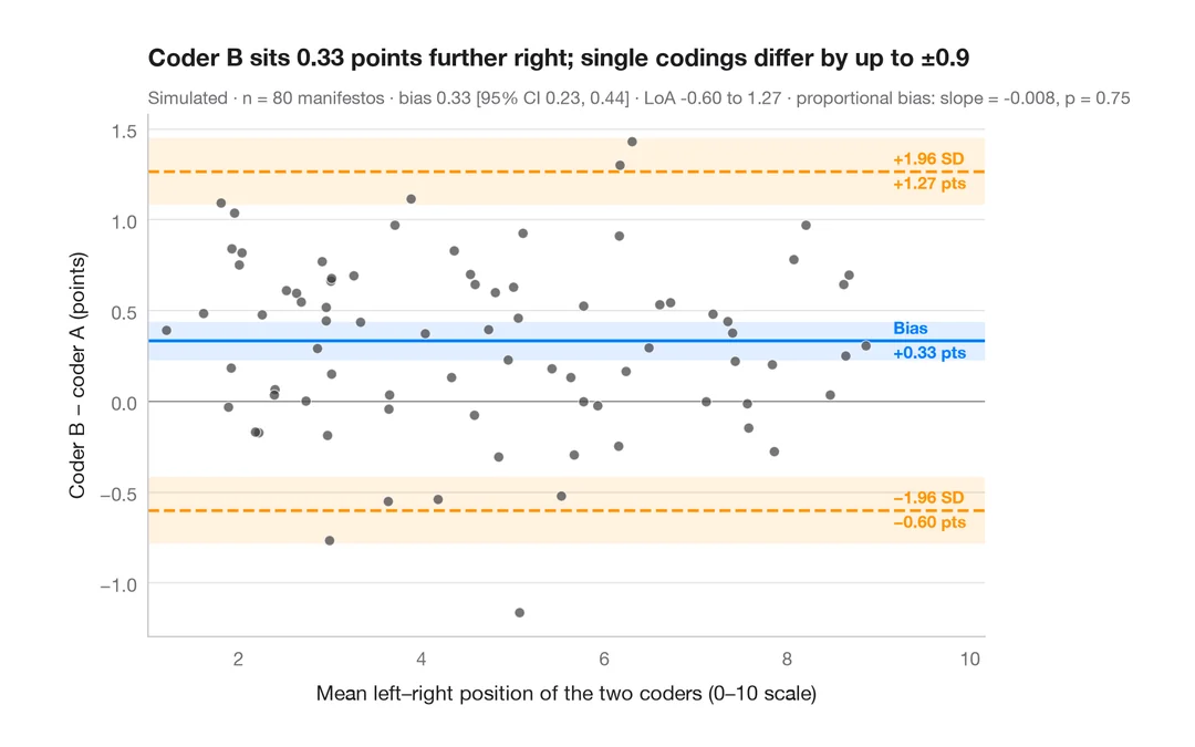

Inference & uncertainty

Bland–Altman plot

Do two coders place party manifestos on the left–right scale the same way? Bias and 95% limits of agreement.

BlandAltmanLeh::bland.altman.plot() / blandr::blandr.draw()