検出力曲線
2標本 t 検定の検出力を、小・中・大の効果量ごとに標本サイズに対して描きます。
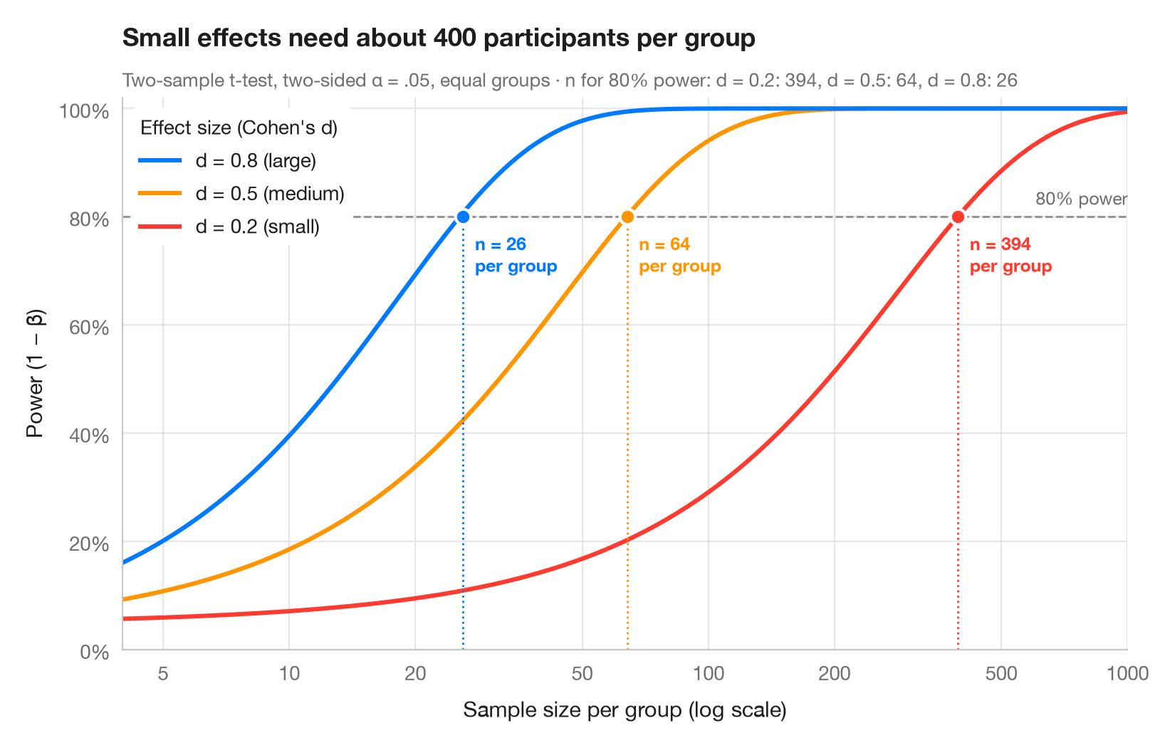
統計的検出力とは、実際に存在する効果を研究が検出できる確率です。各曲線は、コーエンの基準となる効果量(小 d = 0.2、中 0.5、大 0.8)のそれぞれについて、群あたりの参加者数とともに検出力がどう増加するかを示しています。曲線が慣例的な 80% の線を横切る位置に、必要な標本サイズを点で示しています。効果が小さくなるにつれて、必要な標本サイズが急激に膨れ上がることに注目してください(x軸は対数軸です)。
statsmodels.stats.power.TTestIndPower で計算しています。曲線には .power() を、必要な n には .solve_power() を用いています(両側 α = .05、群のサイズは等しいと仮定)。
コードおよび図中のテキストは英語です。
import matplotlib.pyplot as plt
import numpy as np
from matplotlib.ticker import FixedLocator, NullLocator
from statsmodels.stats.power import TTestIndPower

analysis = TTestIndPower()
n = np.geomspace(4, 1000, 300)  # participants per group
effects = {0.2: ("small", "#FF3B30"), 0.5: ("medium", "#FF9500"), 0.8: ("large", "#007AFF")}

fig, ax = plt.subplots(figsize=(8, 5))
ax.axhline(0.8, color="#8E8E93", ls="--", lw=1)
ax.text(1000, 0.815, "80% power", ha="right", va="bottom", fontsize=9, color="#6E6E73")

required = {}
for d, (name, c) in effects.items():
    power = analysis.power(effect_size=d, nobs1=n, alpha=0.05)
    power = np.nan_to_num(power, nan=1.0)  # the noncentral t returns NaN once power ≈ 1
    ax.plot(n, power, color=c, lw=2.2,
            label=f"d = {d} ({name})")
    # Sample size per group that reaches 80% power
    n80 = int(np.ceil(analysis.solve_power(effect_size=d, power=0.8, alpha=0.05)))
    required[d] = n80
    ax.vlines(n80, 0, 0.8, color=c, lw=1, ls=":")
    ax.scatter(n80, 0.8, s=60, color=c, edgecolor="white", lw=1.5, zorder=4)
    ax.annotate(f"n = {n80}\nper group", (n80, 0.8), xytext=(6, -8), textcoords="offset points",
                ha="left", va="top", fontsize=9, color=c, fontweight="semibold")

handles, labels = ax.get_legend_handles_labels()
ax.legend(handles[::-1], labels[::-1], loc="upper left", title="Effect size (Cohen's d)",
          alignment="left", frameon=True, facecolor="white", edgecolor="none", framealpha=1)
ax.set_xscale("log")
ax.xaxis.set_major_locator(FixedLocator([5, 10, 20, 50, 100, 200, 500, 1000]))
ax.xaxis.set_minor_locator(NullLocator())
ax.xaxis.set_major_formatter(lambda v, _: f"{v:g}")
ax.set_xlim(4, 1000)
ax.set_ylim(0, 1.02)
ax.yaxis.set_major_formatter(lambda v, _: f"{v:.0%}")
ax.grid(axis="x")
ax.set_xlabel("Sample size per group (log scale)")
ax.set_ylabel("Power (1 − β)")
ax.set_title("Small effects need about 400 participants per group", pad=26)
ax.text(0, 1.02, "Two-sample t-test, two-sided α = .05, equal groups · n for 80% power: "
        + ", ".join(f"d = {d}: {k}" for d, k in required.items()),
        transform=ax.transAxes, fontsize=9.5, color="#6E6E73")
plt.show()
図にはオプションの PyStatlas スタイル を使用しています。同じ見た目にするには plt.style.use("pystatlas.mplstyle") を追加してください。
引用方法
PyStatlas は Thierry Warin が作成・運営しています。研究や業務に役立った場合は、ぜひ引用してください。
Warin, T. (2026). Power curve. In PyStatlas: A Python Gallery of Statistical Graphics for the Social Sciences. https://warint.github.io/pystatlas/inference-uncertainty/power-curve/
@misc{warin2026statlas,
  author       = {Warin, Thierry},
  title        = {PyStatlas: A Python Gallery of Statistical Graphics for the Social Sciences},
  year         = {2026},
  howpublished = {\url{https://warint.github.io/pystatlas/}},
  note         = {Source code: https://github.com/warint/pystatlas}
}推測と不確実性のその他のグラフ
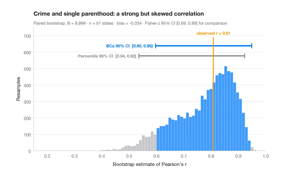
ブートストラップ分布
再標本化した相関係数を、パーセンタイル法と BCa 法の 95% 信頼区間とともに示します。
boot::boot() + boot::boot.ci()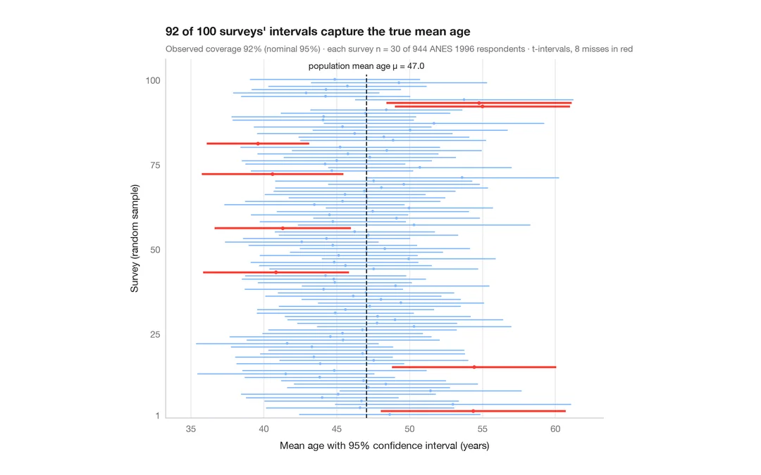
95% 信頼区間の意味
ANES の回答者 944 人から 30 人を抽出する調査を 100 回。平均年齢の 95% 信頼区間のうち真値を外したものを赤で示します。
teaching classic (e.g. TeachingDemos::ci.examp())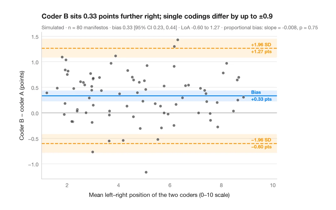
ブランド・アルトマンプロット
2 人のコーダーは政党の選挙綱領を左右軸上に同じように位置づけるか?バイアスと 95% 一致限界。
BlandAltmanLeh::bland.altman.plot() / blandr::blandr.draw()