统计功效曲线
小、中、大效应下双样本 t 检验的统计功效随样本量的变化。
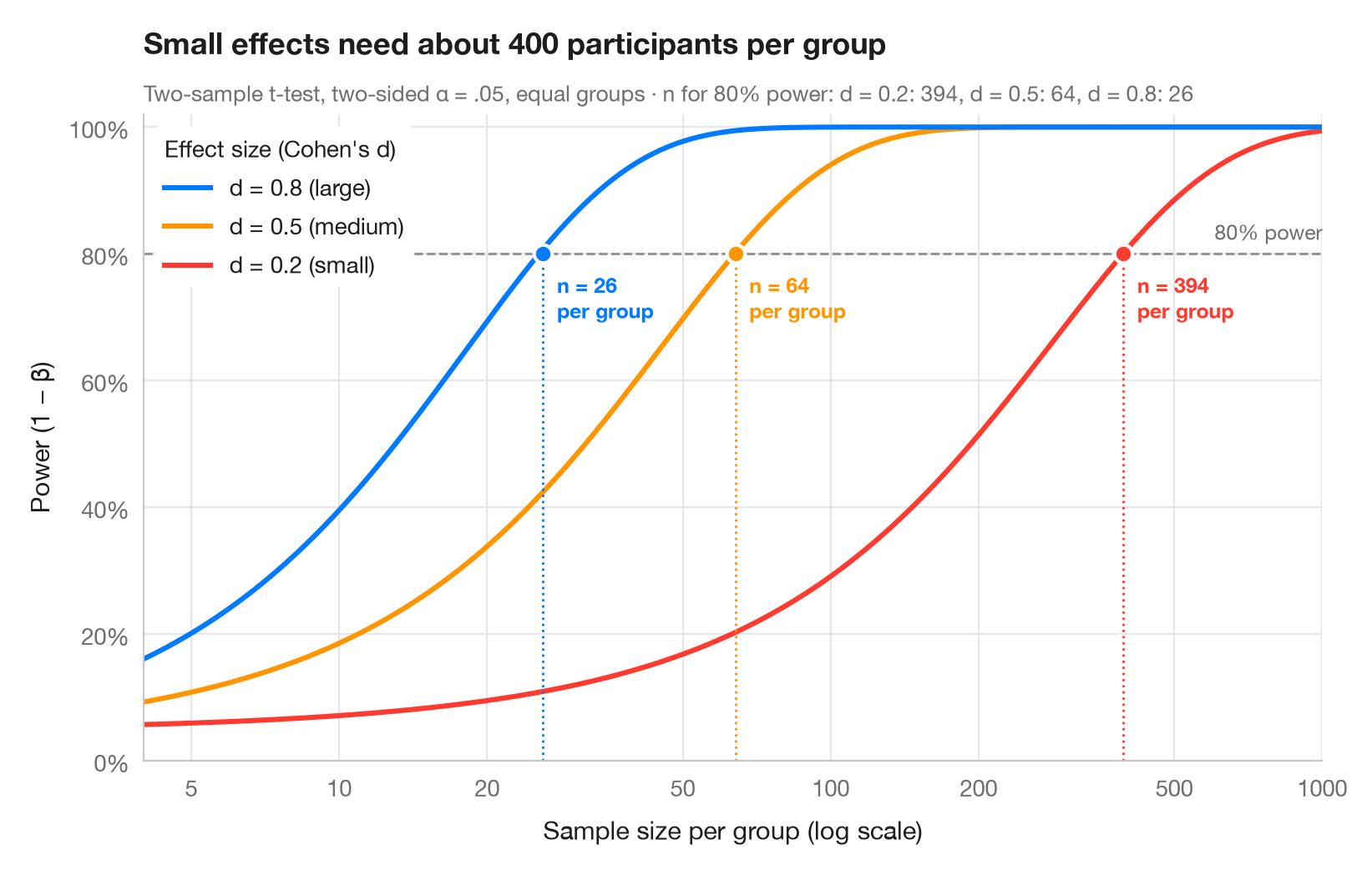
统计功效是一项研究检测到真实存在的效应的概率。每条曲线对应 Cohen 的一个基准效应量(小 d = 0.2、中 0.5、大 0.8),展示功效如何随每组参与者人数增加而提高。曲线与惯用的 80% 线相交处,用圆点标出所需样本量——请注意,随着效应变小,所需样本量会急剧膨胀(x 轴为对数刻度)。
使用 statsmodels.stats.power.TTestIndPower 计算:.power() 绘制曲线,.solve_power() 求所需 n(双侧 α = .05,各组样本量相等)。
代码及图中文字均为英文。
import matplotlib.pyplot as plt
import numpy as np
from matplotlib.ticker import FixedLocator, NullLocator
from statsmodels.stats.power import TTestIndPower

analysis = TTestIndPower()
n = np.geomspace(4, 1000, 300)  # participants per group
effects = {0.2: ("small", "#FF3B30"), 0.5: ("medium", "#FF9500"), 0.8: ("large", "#007AFF")}

fig, ax = plt.subplots(figsize=(8, 5))
ax.axhline(0.8, color="#8E8E93", ls="--", lw=1)
ax.text(1000, 0.815, "80% power", ha="right", va="bottom", fontsize=9, color="#6E6E73")

required = {}
for d, (name, c) in effects.items():
    power = analysis.power(effect_size=d, nobs1=n, alpha=0.05)
    power = np.nan_to_num(power, nan=1.0)  # the noncentral t returns NaN once power ≈ 1
    ax.plot(n, power, color=c, lw=2.2,
            label=f"d = {d} ({name})")
    # Sample size per group that reaches 80% power
    n80 = int(np.ceil(analysis.solve_power(effect_size=d, power=0.8, alpha=0.05)))
    required[d] = n80
    ax.vlines(n80, 0, 0.8, color=c, lw=1, ls=":")
    ax.scatter(n80, 0.8, s=60, color=c, edgecolor="white", lw=1.5, zorder=4)
    ax.annotate(f"n = {n80}\nper group", (n80, 0.8), xytext=(6, -8), textcoords="offset points",
                ha="left", va="top", fontsize=9, color=c, fontweight="semibold")

handles, labels = ax.get_legend_handles_labels()
ax.legend(handles[::-1], labels[::-1], loc="upper left", title="Effect size (Cohen's d)",
          alignment="left", frameon=True, facecolor="white", edgecolor="none", framealpha=1)
ax.set_xscale("log")
ax.xaxis.set_major_locator(FixedLocator([5, 10, 20, 50, 100, 200, 500, 1000]))
ax.xaxis.set_minor_locator(NullLocator())
ax.xaxis.set_major_formatter(lambda v, _: f"{v:g}")
ax.set_xlim(4, 1000)
ax.set_ylim(0, 1.02)
ax.yaxis.set_major_formatter(lambda v, _: f"{v:.0%}")
ax.grid(axis="x")
ax.set_xlabel("Sample size per group (log scale)")
ax.set_ylabel("Power (1 − β)")
ax.set_title("Small effects need about 400 participants per group", pad=26)
ax.text(0, 1.02, "Two-sample t-test, two-sided α = .05, equal groups · n for 80% power: "
        + ", ".join(f"d = {d}: {k}" for d, k in required.items()),
        transform=ax.transAxes, fontsize=9.5, color="#6E6E73")
plt.show()
图表使用了可选的 PyStatlas 样式:添加 plt.style.use("pystatlas.mplstyle") 即可完全还原其外观。
如何引用
PyStatlas 由 Thierry Warin 创建并维护。如果它对你的工作有所帮助,敬请引用。
Warin, T. (2026). Power curve. In PyStatlas: A Python Gallery of Statistical Graphics for the Social Sciences. https://warint.github.io/pystatlas/inference-uncertainty/power-curve/
@misc{warin2026statlas,
  author       = {Warin, Thierry},
  title        = {PyStatlas: A Python Gallery of Statistical Graphics for the Social Sciences},
  year         = {2026},
  howpublished = {\url{https://warint.github.io/pystatlas/}},
  note         = {Source code: https://github.com/warint/pystatlas}
}更多推断与不确定性图表
推断与不确定性
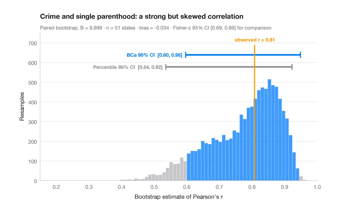
自助法分布
重抽样得到的相关系数,附百分位数法和 BCa 95% 置信区间。
boot::boot() + boot::boot.ci()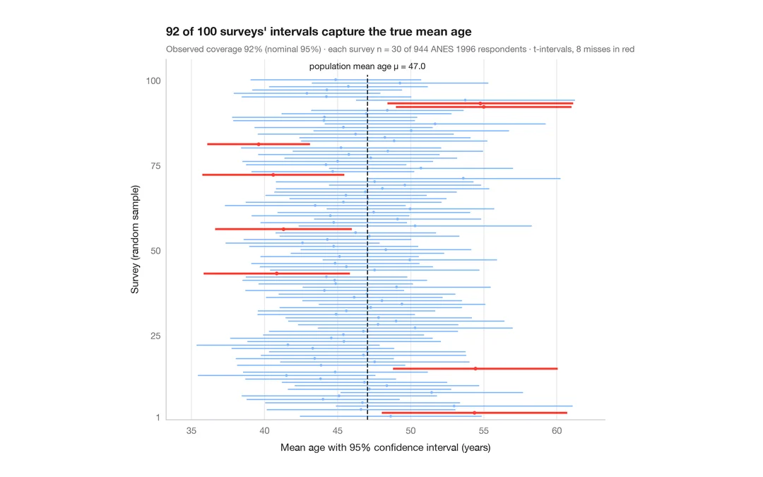
推断与不确定性
95% 置信区间的含义
从 944 名 ANES 受访者中抽取 30 人,重复调查 100 次;未覆盖真值的平均年龄 95% 置信区间以红色显示。
teaching classic (e.g. TeachingDemos::ci.examp())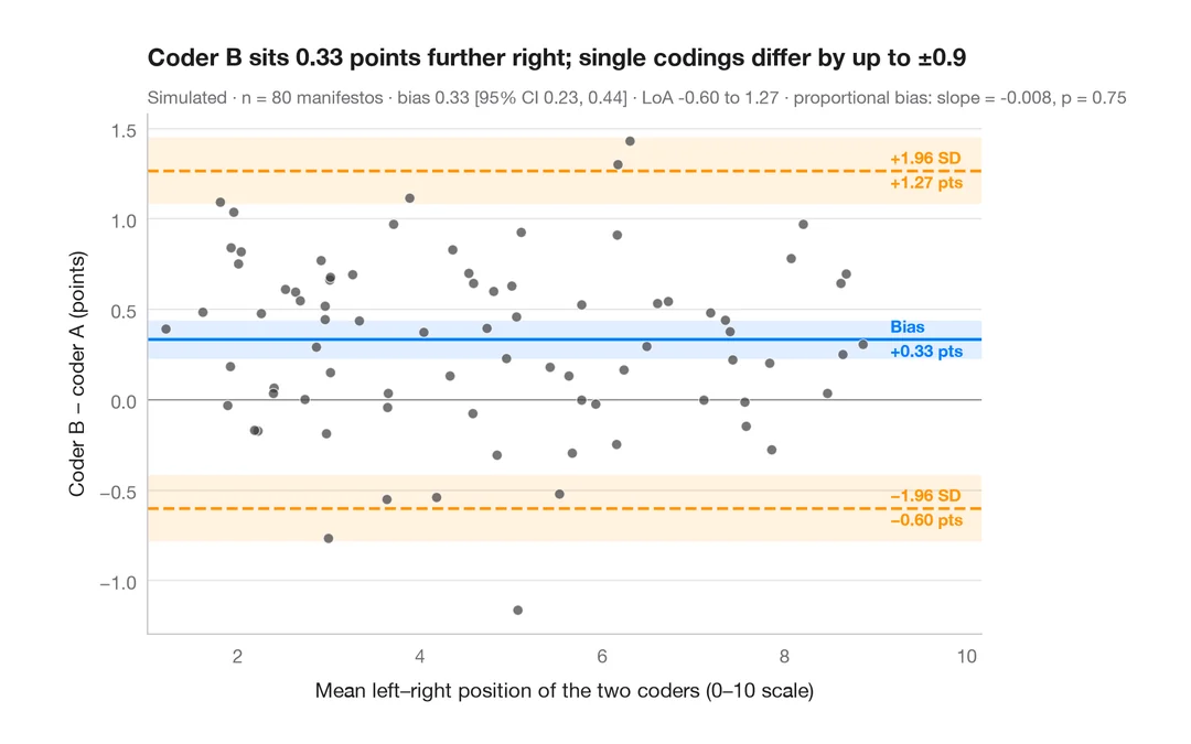
推断与不确定性
Bland–Altman 图
两位编码员对政党竞选纲领左右立场的定位是否一致?偏差与 95% 一致性界限。
BlandAltmanLeh::bland.altman.plot() / blandr::blandr.draw()