Bland–Altman 图
两位编码员对政党竞选纲领左右立场的定位是否一致?偏差与 95% 一致性界限。
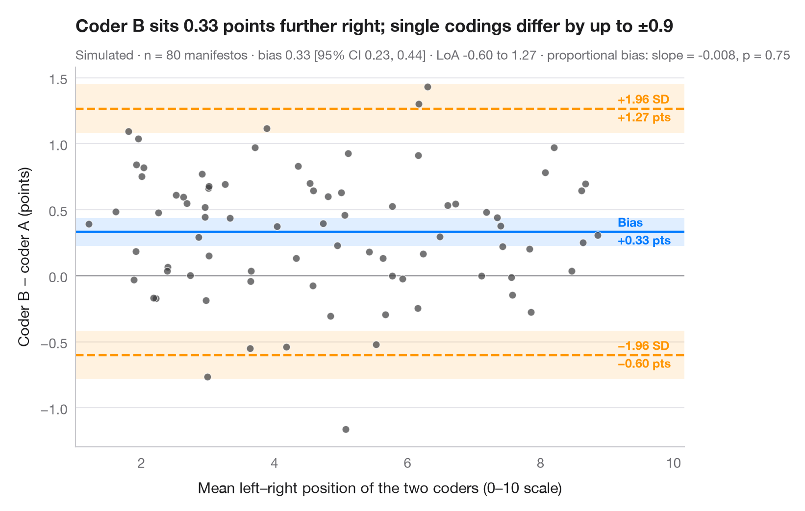
当两种仪器——或两位编码员——测量同一事物时,高相关并不能说明它们是否一致。Bland–Altman 图以两种方法之差为纵轴、两者均值为横轴。中间的线是平均差(系统偏差),外侧两条线是 95% 一致性界限(偏差 ± 1.96 SD),大多数分歧落在其中。阴影带是这三条线的 95% 置信区间,使用 Bland 和 Altman (1986) 的标准误;点云若呈现斜率,则提示存在比例偏差。
数据由 numpy(固定种子)模拟,模仿内容分析中的经典检验:两位受过训练的编码员分别将同样 80 份政党竞选纲领定位在 0–10 的左右量表上,编码员 B 被设定为比编码员 A 平均偏右约 0.4 分。偏差和区间使用 scipy.stats.t;斜率检验是 statsmodels 的 OLS 拟合。
代码及图中文字均为英文。
import matplotlib.pyplot as plt
import numpy as np
import statsmodels.api as sm
from scipy import stats

# Simulated coding: 80 manifestos placed on a 0–10 left–right scale by two coders;
# coder B leans ~0.4 points to the right and is a little noisier
rng = np.random.default_rng(11)
n = 80
position = rng.uniform(1.5, 8.5, n)
coder_a = position + rng.normal(0, 0.35, n)
coder_b = position + 0.4 + rng.normal(0, 0.45, n)

mean, diff = (coder_a + coder_b) / 2, coder_b - coder_a
bias, sd = diff.mean(), diff.std(ddof=1)
loa = bias + np.array([-1.96, 1.96]) * sd
t = stats.t.ppf(0.975, n - 1)
ci_bias = t * sd / np.sqrt(n)            # half-width of the CI for the bias
ci_loa = t * np.sqrt(3 * sd**2 / n)      # Bland & Altman (1986) SE of a limit
slope = sm.OLS(diff, sm.add_constant(mean)).fit()

fig, ax = plt.subplots(figsize=(8, 5))
for y0, hw, c in [(bias, ci_bias, "#007AFF"), (loa[0], ci_loa, "#FF9500"), (loa[1], ci_loa, "#FF9500")]:
    ax.axhspan(y0 - hw, y0 + hw, color=c, alpha=0.12, lw=0)
    ax.axhline(y0, color=c, lw=1.6, ls="-" if c == "#007AFF" else "--")
ax.axhline(0, color="#8E8E93", lw=0.8)
ax.scatter(mean, diff, s=30, color="#3A3A3C", alpha=0.7, edgecolor="white", lw=0.6, zorder=3)

# Labels on the right margin
x_lab = mean.max() + 0.3
for y0, name, c in [(loa[1], "+1.96 SD", "#FF9500"), (bias, "Bias", "#007AFF"),
                    (loa[0], "−1.96 SD", "#FF9500")]:
    ax.text(x_lab, y0, f"{name}\n{y0:+.2f} pts".replace("-", "−"), va="center", ha="left", fontsize=9,
            color=c, fontweight="semibold", linespacing=1.3)

ax.set_xlim(mean.min() - 0.2, mean.max() + 1.3)
ax.set_xlabel("Mean left–right position of the two coders (0–10 scale)")
ax.set_ylabel("Coder B − coder A (points)")
ax.set_title(f"Coder B sits {bias:.2f} points further right; single codings differ "
             f"by up to ±{1.96 * sd:.1f}", pad=26)
ax.text(0, 1.02, f"Simulated · n = {n} manifestos · bias {bias:.2f} [95% CI {bias - ci_bias:.2f}, "
        f"{bias + ci_bias:.2f}] · LoA {loa[0]:.2f} to {loa[1]:.2f} · proportional bias: slope = {slope.params[1]:.3f}, "
        f"p = {slope.pvalues[1]:.2f}", transform=ax.transAxes, fontsize=9.5, color="#6E6E73")
plt.show()
图表使用了可选的 PyStatlas 样式:添加 plt.style.use("pystatlas.mplstyle") 即可完全还原其外观。
数据来源
- Simulated data. Simulated data with a fixed random seed, created for this example.
No real respondents, documents or measurements: the numbers only illustrate how the chart and its statistics work.
这些示例用于说明统计方法。图表标题描述的是该图在这些特定数据中呈现的内容——这些数据往往样本较小、年代较早或并不完整——而不是作者对实质问题的立场。关于解释、背景和数据质量,请以此处引用的原始来源为准。
如何引用
PyStatlas 由 Thierry Warin 创建并维护。如果它对你的工作有所帮助,敬请引用。
Warin, T. (2026). Bland–Altman plot. In PyStatlas: A Python Gallery of Statistical Graphics for the Social Sciences. https://warint.github.io/pystatlas/inference-uncertainty/bland-altman/
@misc{warin2026statlas,
  author       = {Warin, Thierry},
  title        = {PyStatlas: A Python Gallery of Statistical Graphics for the Social Sciences},
  year         = {2026},
  howpublished = {\url{https://warint.github.io/pystatlas/}},
  note         = {Source code: https://github.com/warint/pystatlas}
}