元分析森林图
教师期望能否提高学生的智商?19 项“皮格马利翁”实验、随机效应合并估计菱形与异质性统计量。
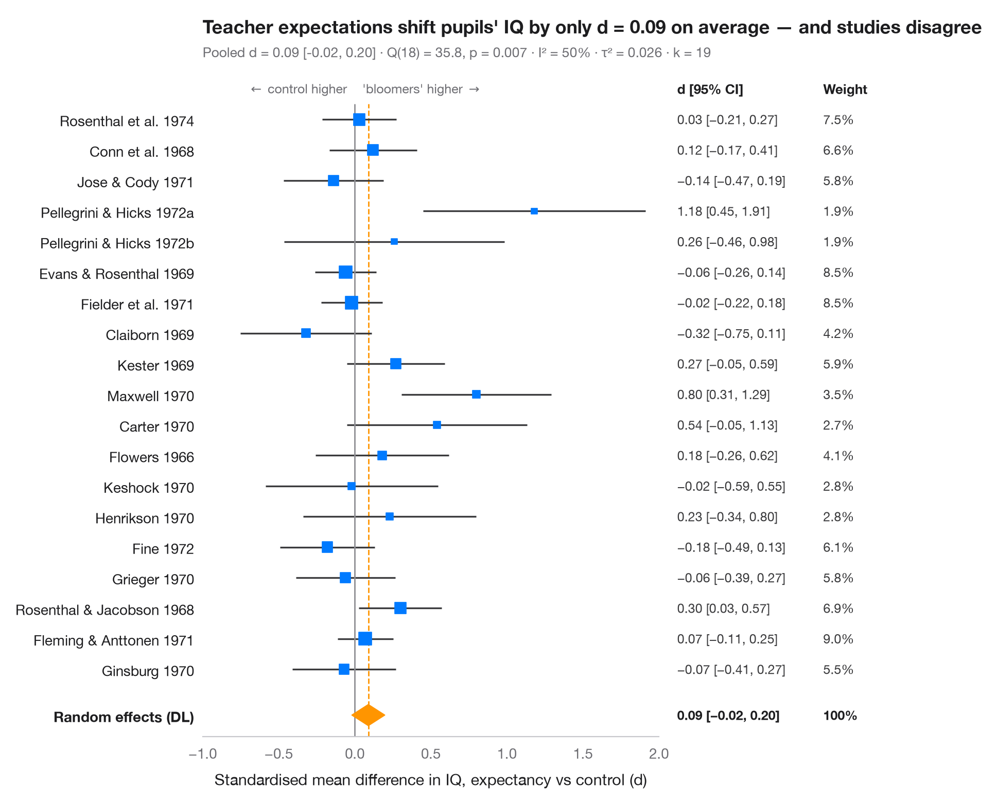
森林图将元分析中的每项研究排成一行:方块是该研究的估计值(面积与研究权重成正比),须线是其 95% 置信区间。底部的菱形是随机效应(DerSimonian–Laird)合并估计,其宽度即 95% 置信区间。副标题报告异质性——Cochran Q、I²(由研究间真实差异造成的变异占比)和 τ²(其方差)。
数据为 Raudenbush (1984) 综合的 19 项教师期望(“皮格马利翁”)实验:每项实验都告诉教师某些学生即将“开窍”,随后将这些学生的智商与对照组比较。效应量为标准化均值差(d > 0:被认为“开窍”的学生得分更高)及其抽样方差,按 R 包 metafor 中 dat.raudenbush1985 公布的数值录入。合并使用 statsmodels.stats.meta_analysis 中的 combine_effects。平均效应很小且置信区间包含零,而各研究之间的差异超出了偶然所能解释的范围;Raudenbush 将这种差异很大程度上归因于在诱导期望之前教师认识学生的时间长短。
代码及图中文字均为英文。
import matplotlib.pyplot as plt
import numpy as np
import pandas as pd
from matplotlib.transforms import blended_transform_factory
from scipy import stats
from statsmodels.stats.meta_analysis import combine_effects

# Teacher-expectancy experiments (Raudenbush, 1984): standardised mean difference
# in pupil IQ (yi) and its sampling variance (vi), as in metafor's dat.raudenbush1985
pyg = pd.DataFrame({
    "study": ["Rosenthal et al. 1974", "Conn et al. 1968", "Jose & Cody 1971",
              "Pellegrini & Hicks 1972a", "Pellegrini & Hicks 1972b", "Evans & Rosenthal 1969",
              "Fielder et al. 1971", "Claiborn 1969", "Kester 1969", "Maxwell 1970", "Carter 1970",
              "Flowers 1966", "Keshock 1970", "Henrikson 1970", "Fine 1972", "Grieger 1970",
              "Rosenthal & Jacobson 1968", "Fleming & Anttonen 1971", "Ginsburg 1970"],
    "yi": [0.03, 0.12, -0.14, 1.18, 0.26, -0.06, -0.02, -0.32, 0.27, 0.80, 0.54, 0.18, -0.02,
           0.23, -0.18, -0.06, 0.30, 0.07, -0.07],
    "vi": [0.0156, 0.0216, 0.0279, 0.1391, 0.1362, 0.0106, 0.0106, 0.0484, 0.0269, 0.0630,
           0.0912, 0.0497, 0.0835, 0.0841, 0.0253, 0.0279, 0.0193, 0.0088, 0.0303]})
res = combine_effects(pyg.yi, pyg.vi, method_re="dl", row_names=pyg.study)
tab = res.summary_frame()
studies, pooled = tab.iloc[:len(pyg)], tab.loc["random effect"]
q_p = stats.chi2.sf(res.q, res.df_resid)

fig, ax = plt.subplots(figsize=(8, 7.6))
y = np.arange(len(pyg), 0, -1) + 1.0
ax.hlines(y, studies.ci_low, studies.ci_upp, color="#3A3A3C", lw=1.2)
ax.scatter(studies.eff, y, marker="s", s=900 * studies.w_re, color="#007AFF", zorder=3)

# Pooled random-effects diamond
lo, mid, hi = pooled.ci_low, pooled.eff, pooled.ci_upp
ax.fill([lo, mid, hi, mid], [0.5, 0.85, 0.5, 0.15], color="#FF9500", zorder=3)
ax.vlines(0, -0.2, len(pyg) + 1.5, color="#8E8E93", lw=1)
ax.vlines(mid, -0.2, len(pyg) + 1.5, color="#FF9500", lw=1, ls="--", zorder=1)

# Table columns to the right of the plot: d [95% CI] and weight
tr = blended_transform_factory(ax.transAxes, ax.transData)
for x, head in [(1.04, "d [95% CI]"), (1.36, "Weight")]:
    ax.text(x, len(pyg) + 2, head, transform=tr, fontsize=9.5, fontweight="semibold", va="center")
for yi, (_, r) in zip(y, studies.iterrows()):
    ax.text(1.04, yi, f"{r.eff:.2f} [{r.ci_low:.2f}, {r.ci_upp:.2f}]".replace("-", "−"),
            transform=tr, fontsize=9, va="center", color="#3A3A3C")
    ax.text(1.36, yi, f"{100 * r.w_re:.1f}%", transform=tr, fontsize=9, va="center", color="#3A3A3C")
for x, txt in [(1.04, f"{mid:.2f} [{lo:.2f}, {hi:.2f}]".replace("-", "−")), (1.36, "100%")]:
    ax.text(x, 0.5, txt, transform=tr, fontsize=9, va="center", fontweight="semibold")

ax.set_xlim(-1.0, 2.0)
ax.set_yticks(list(y) + [0.5], list(pyg.study) + ["Random effects (DL)"])
ax.get_yticklabels()[-1].set_fontweight("semibold")
ax.set_ylim(-0.2, len(pyg) + 2.6)
ax.grid(False); ax.spines["left"].set_visible(False)
ax.set_xlabel("Standardised mean difference in IQ, expectancy vs control (d)")
ax.text(-0.05, len(pyg) + 2, r"$\leftarrow$ control higher", ha="right", va="center", fontsize=9, color="#6E6E73")
ax.text(0.05, len(pyg) + 2, r"'bloomers' higher $\rightarrow$", ha="left", va="center", fontsize=9, color="#6E6E73")
ax.tick_params(axis="y", labelcolor="#1D1D1F")
ax.set_title(f"Teacher expectations shift pupils' IQ by only d = {mid:.2f} on average — "
             "and studies disagree", pad=26)
ax.text(0, 1.02, f"Pooled d = {mid:.2f} [{lo:.2f}, {hi:.2f}] · Q({res.df_resid:.0f}) = "
        f"{res.q:.1f}, p = {q_p:.3f} · I² = {100 * res.i2:.0f}% · τ² = {res.tau2:.3f} · k = {len(pyg)}",
        transform=ax.transAxes, fontsize=9.5, color="#6E6E73")
plt.show()
图表使用了可选的 PyStatlas 样式:添加 plt.style.use("pystatlas.mplstyle") 即可完全还原其外观。
数据来源
- Teacher-expectancy experiments (Raudenbush, 1984). Raudenbush, S. W. (1984). Magnitude of teacher expectancy effects on pupil IQ as a function of the credibility of expectancy induction: A synthesis of findings from 18 experiments. Journal of Educational Psychology, 76(1), 85–97. https://doi.org/10.1037/0022-0663.76.1.85
Effect sizes and variances typed in from dat.raudenbush1985 in R's metadat/metafor (Viechtbauer, 2010, Journal of Statistical Software, 36(3), https://doi.org/10.18637/jss.v036.i03); one of the 18 experiments contributes two rows.
这些示例用于说明统计方法。图表标题描述的是该图在这些特定数据中呈现的内容——这些数据往往样本较小、年代较早或并不完整——而不是作者对实质问题的立场。关于解释、背景和数据质量,请以此处引用的原始来源为准。
如何引用
PyStatlas 由 Thierry Warin 创建并维护。如果它对你的工作有所帮助,敬请引用。
Warin, T. (2026). Meta-analysis forest plot. In PyStatlas: A Python Gallery of Statistical Graphics for the Social Sciences. https://warint.github.io/pystatlas/inference-uncertainty/meta-analysis-forest/
@misc{warin2026statlas,
  author       = {Warin, Thierry},
  title        = {PyStatlas: A Python Gallery of Statistical Graphics for the Social Sciences},
  year         = {2026},
  howpublished = {\url{https://warint.github.io/pystatlas/}},
  note         = {Source code: https://github.com/warint/pystatlas}
}