漏斗图
小型“皮格马利翁”研究是否更乐观?19 个教师期望效应对其标准误作图,附伪 95% 漏斗和 Egger 检验。
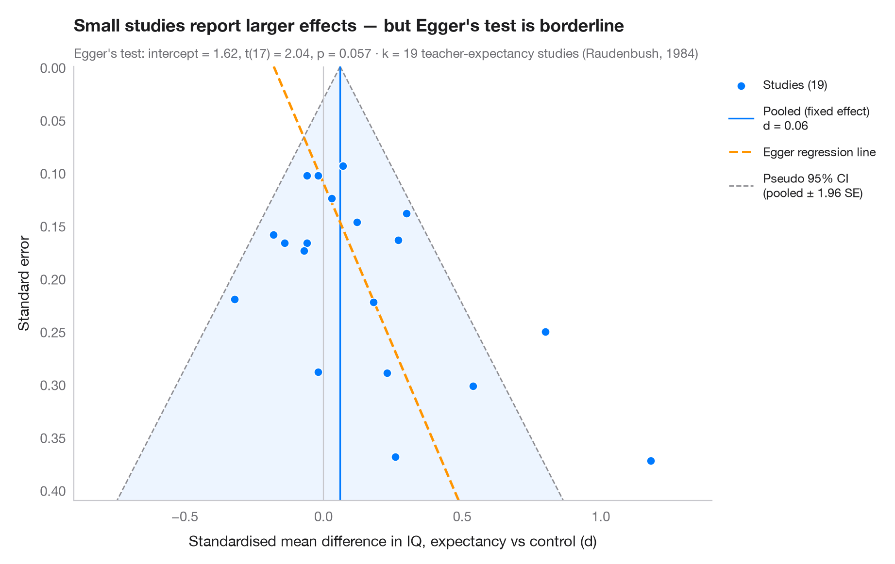
每个点是一项研究:横轴为效应量,纵轴(倒置)为标准误,因此大型、精确的研究位于上方。若无偏倚,各点围绕合并效应形成对称的漏斗,其中 95% 落在伪置信区域(± 1.96 SE)内。如果结果为零或为负的小型研究缺失——即发表偏倚——漏斗底部就会失衡。Egger 回归检验(标准正态离差对精度回归)量化这种不对称;其拟合线以虚线表示。
数据为 Raudenbush (1984) 的 19 项教师期望(“皮格马利翁”)实验:学生智商的标准化均值差及其抽样方差,按 R 包 metafor 中 dat.raudenbush1985 公布的数值录入。精度最低的研究报告了最大的效应,Egger 截距处于显著性边缘。不对称并不能证明存在发表偏倚:这里的小型研究大多是教师认识学生一周或更短时间的研究,而 Raudenbush 证明这种情况确实会产生更大的效应。Egger 检验是 statsmodels 的 OLS 拟合。
代码及图中文字均为英文。
import matplotlib.pyplot as plt
import numpy as np
import statsmodels.api as sm

# Teacher-expectancy experiments (Raudenbush, 1984): standardised mean difference
# in pupil IQ and its sampling variance, as in metafor's dat.raudenbush1985
dp = np.array([0.03, 0.12, -0.14, 1.18, 0.26, -0.06, -0.02, -0.32, 0.27, 0.80, 0.54, 0.18,
               -0.02, 0.23, -0.18, -0.06, 0.30, 0.07, -0.07])
vi = np.array([0.0156, 0.0216, 0.0279, 0.1391, 0.1362, 0.0106, 0.0106, 0.0484, 0.0269, 0.0630,
               0.0912, 0.0497, 0.0835, 0.0841, 0.0253, 0.0279, 0.0193, 0.0088, 0.0303])
sp = np.sqrt(vi)

# Fixed-effect pooled estimate and Egger's test: z = b0 + b1 · precision
w = 1 / sp**2
pooled = np.sum(w * dp) / w.sum()
egger = sm.OLS(dp / sp, sm.add_constant(1 / sp)).fit()
b0, b1 = egger.params

fig, ax = plt.subplots(figsize=(9, 5.6))
s_grid = np.linspace(0, sp.max() * 1.1, 100)
ax.fill_betweenx(s_grid, pooled - 1.96 * s_grid, pooled + 1.96 * s_grid, color="#007AFF",
                 alpha=0.07, lw=0)
for sign in (-1, 1):
    ax.plot(pooled + sign * 1.96 * s_grid, s_grid, color="#8E8E93", lw=1, ls="--",
            label="Pseudo 95% CI\n(pooled ± 1.96 SE)" if sign > 0 else None)
ax.axvline(pooled, color="#007AFF", lw=1.2, label=f"Pooled (fixed effect)\nd = {pooled:.2f}")
ax.axvline(0, color="#C7C7CC", lw=0.8)
ax.plot(b1 + b0 * s_grid, s_grid, color="#FF9500", lw=1.8, ls="--", label="Egger regression line")

ax.scatter(dp, sp, s=40, color="#007AFF", edgecolor="white", lw=0.7, zorder=3,
           label=f"Studies ({len(dp)})")

ax.invert_yaxis()
ax.set_ylim(sp.max() * 1.1, 0)
ax.set_xlim(-0.9, 1.4)
ax.set_xlabel("Standardised mean difference in IQ, expectancy vs control (d)")
ax.set_ylabel("Standard error")
ax.grid(axis="y", visible=False)

handles, labels = ax.get_legend_handles_labels()
order = [3, 1, 2, 0]
ax.legend([handles[i] for i in order], [labels[i] for i in order], loc="upper left",
          bbox_to_anchor=(1.01, 1), fontsize=9, labelspacing=1)

ax.set_title("Small studies report larger effects — " + ("Egger's test flags asymmetry"
             if egger.pvalues[0] < 0.05 else "but Egger's test is borderline"), pad=26)
ax.text(0, 1.02, f"Egger's test: intercept = {b0:.2f}, t({egger.df_resid:.0f}) = "
        f"{egger.tvalues[0]:.2f}, p = {egger.pvalues[0]:.3f} · k = {len(dp)} teacher-expectancy "
        f"studies (Raudenbush, 1984)", transform=ax.transAxes, fontsize=9.5, color="#6E6E73")
plt.show()
图表使用了可选的 PyStatlas 样式:添加 plt.style.use("pystatlas.mplstyle") 即可完全还原其外观。
数据来源
- Teacher-expectancy experiments (Raudenbush, 1984). Raudenbush, S. W. (1984). Magnitude of teacher expectancy effects on pupil IQ as a function of the credibility of expectancy induction: A synthesis of findings from 18 experiments. Journal of Educational Psychology, 76(1), 85–97. https://doi.org/10.1037/0022-0663.76.1.85
Effect sizes and variances typed in from dat.raudenbush1985 in R's metadat/metafor (Viechtbauer, 2010, Journal of Statistical Software, 36(3), https://doi.org/10.18637/jss.v036.i03); one of the 18 experiments contributes two rows.
这些示例用于说明统计方法。图表标题描述的是该图在这些特定数据中呈现的内容——这些数据往往样本较小、年代较早或并不完整——而不是作者对实质问题的立场。关于解释、背景和数据质量,请以此处引用的原始来源为准。
如何引用
PyStatlas 由 Thierry Warin 创建并维护。如果它对你的工作有所帮助,敬请引用。
Warin, T. (2026). Funnel plot. In PyStatlas: A Python Gallery of Statistical Graphics for the Social Sciences. https://warint.github.io/pystatlas/inference-uncertainty/funnel-plot/
@misc{warin2026statlas,
  author       = {Warin, Thierry},
  title        = {PyStatlas: A Python Gallery of Statistical Graphics for the Social Sciences},
  year         = {2026},
  howpublished = {\url{https://warint.github.io/pystatlas/}},
  note         = {Source code: https://github.com/warint/pystatlas}
}