メタアナリシスのフォレストプロット
教師の期待は児童の IQ を高めるか?19 件の「ピグマリオン」実験、変量効果による統合推定のひし形と異質性の統計量。
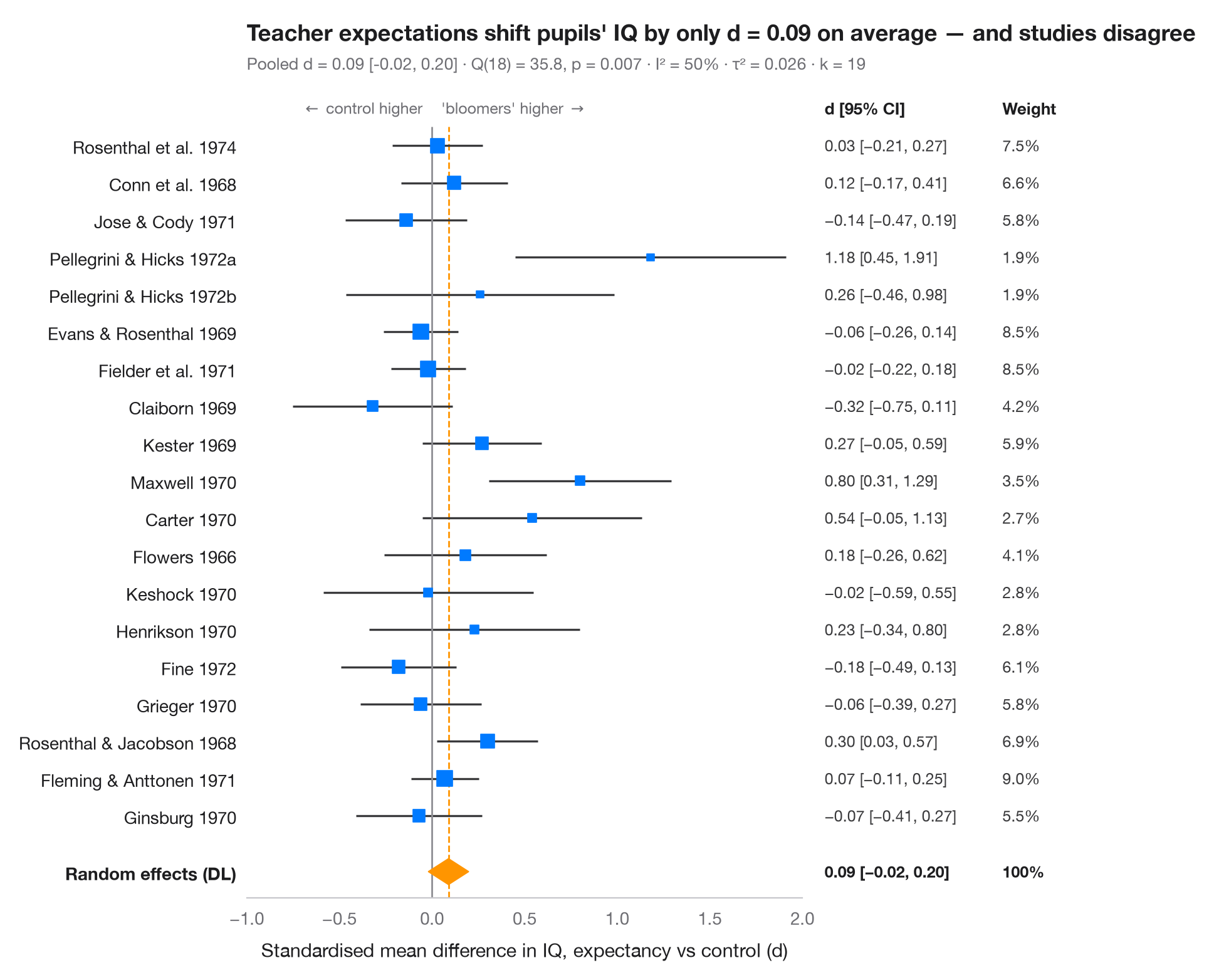
フォレストプロットは、メタアナリシスに含まれる各研究を 1 行ずつ並べます。四角は研究の推定値(面積は研究の重みに比例)、ひげはその 95% 信頼区間です。下端のひし形は変量効果(DerSimonian–Laird)による統合推定値で、その幅が 95% 信頼区間を表します。サブタイトルには異質性 — Cochran の Q、I²(研究間の真の差に起因するばらつきの割合)、τ²(その分散)— を示しています。
データは Raudenbush (1984) が統合した教師期待(「ピグマリオン」)実験 19 件です。各実験では、一部の児童がまもなく「伸びる」と教師に伝え、後にその児童の IQ を対照群と比較しました。効果量は標準化平均差(d > 0:「伸びる」とされた児童の得点が高い)とその標本分散で、R の metafor の dat.raudenbush1985 に公表された値をそのまま入力しています。統合には statsmodels.stats.meta_analysis の combine_effects を使います。平均効果は小さく信頼区間はゼロを含む一方、研究間のばらつきは偶然で説明できる以上に大きく、Raudenbush はその多くを、期待を誘導する前に教師が児童をどれだけ長く知っていたかに帰しました。
コードおよび図中のテキストは英語です。
import matplotlib.pyplot as plt
import numpy as np
import pandas as pd
from matplotlib.transforms import blended_transform_factory
from scipy import stats
from statsmodels.stats.meta_analysis import combine_effects

# Teacher-expectancy experiments (Raudenbush, 1984): standardised mean difference
# in pupil IQ (yi) and its sampling variance (vi), as in metafor's dat.raudenbush1985
pyg = pd.DataFrame({
    "study": ["Rosenthal et al. 1974", "Conn et al. 1968", "Jose & Cody 1971",
              "Pellegrini & Hicks 1972a", "Pellegrini & Hicks 1972b", "Evans & Rosenthal 1969",
              "Fielder et al. 1971", "Claiborn 1969", "Kester 1969", "Maxwell 1970", "Carter 1970",
              "Flowers 1966", "Keshock 1970", "Henrikson 1970", "Fine 1972", "Grieger 1970",
              "Rosenthal & Jacobson 1968", "Fleming & Anttonen 1971", "Ginsburg 1970"],
    "yi": [0.03, 0.12, -0.14, 1.18, 0.26, -0.06, -0.02, -0.32, 0.27, 0.80, 0.54, 0.18, -0.02,
           0.23, -0.18, -0.06, 0.30, 0.07, -0.07],
    "vi": [0.0156, 0.0216, 0.0279, 0.1391, 0.1362, 0.0106, 0.0106, 0.0484, 0.0269, 0.0630,
           0.0912, 0.0497, 0.0835, 0.0841, 0.0253, 0.0279, 0.0193, 0.0088, 0.0303]})
res = combine_effects(pyg.yi, pyg.vi, method_re="dl", row_names=pyg.study)
tab = res.summary_frame()
studies, pooled = tab.iloc[:len(pyg)], tab.loc["random effect"]
q_p = stats.chi2.sf(res.q, res.df_resid)

fig, ax = plt.subplots(figsize=(8, 7.6))
y = np.arange(len(pyg), 0, -1) + 1.0
ax.hlines(y, studies.ci_low, studies.ci_upp, color="#3A3A3C", lw=1.2)
ax.scatter(studies.eff, y, marker="s", s=900 * studies.w_re, color="#007AFF", zorder=3)

# Pooled random-effects diamond
lo, mid, hi = pooled.ci_low, pooled.eff, pooled.ci_upp
ax.fill([lo, mid, hi, mid], [0.5, 0.85, 0.5, 0.15], color="#FF9500", zorder=3)
ax.vlines(0, -0.2, len(pyg) + 1.5, color="#8E8E93", lw=1)
ax.vlines(mid, -0.2, len(pyg) + 1.5, color="#FF9500", lw=1, ls="--", zorder=1)

# Table columns to the right of the plot: d [95% CI] and weight
tr = blended_transform_factory(ax.transAxes, ax.transData)
for x, head in [(1.04, "d [95% CI]"), (1.36, "Weight")]:
    ax.text(x, len(pyg) + 2, head, transform=tr, fontsize=9.5, fontweight="semibold", va="center")
for yi, (_, r) in zip(y, studies.iterrows()):
    ax.text(1.04, yi, f"{r.eff:.2f} [{r.ci_low:.2f}, {r.ci_upp:.2f}]".replace("-", "−"),
            transform=tr, fontsize=9, va="center", color="#3A3A3C")
    ax.text(1.36, yi, f"{100 * r.w_re:.1f}%", transform=tr, fontsize=9, va="center", color="#3A3A3C")
for x, txt in [(1.04, f"{mid:.2f} [{lo:.2f}, {hi:.2f}]".replace("-", "−")), (1.36, "100%")]:
    ax.text(x, 0.5, txt, transform=tr, fontsize=9, va="center", fontweight="semibold")

ax.set_xlim(-1.0, 2.0)
ax.set_yticks(list(y) + [0.5], list(pyg.study) + ["Random effects (DL)"])
ax.get_yticklabels()[-1].set_fontweight("semibold")
ax.set_ylim(-0.2, len(pyg) + 2.6)
ax.grid(False); ax.spines["left"].set_visible(False)
ax.set_xlabel("Standardised mean difference in IQ, expectancy vs control (d)")
ax.text(-0.05, len(pyg) + 2, r"$\leftarrow$ control higher", ha="right", va="center", fontsize=9, color="#6E6E73")
ax.text(0.05, len(pyg) + 2, r"'bloomers' higher $\rightarrow$", ha="left", va="center", fontsize=9, color="#6E6E73")
ax.tick_params(axis="y", labelcolor="#1D1D1F")
ax.set_title(f"Teacher expectations shift pupils' IQ by only d = {mid:.2f} on average — "
             "and studies disagree", pad=26)
ax.text(0, 1.02, f"Pooled d = {mid:.2f} [{lo:.2f}, {hi:.2f}] · Q({res.df_resid:.0f}) = "
        f"{res.q:.1f}, p = {q_p:.3f} · I² = {100 * res.i2:.0f}% · τ² = {res.tau2:.3f} · k = {len(pyg)}",
        transform=ax.transAxes, fontsize=9.5, color="#6E6E73")
plt.show()
図にはオプションの PyStatlas スタイル を使用しています。同じ見た目にするには plt.style.use("pystatlas.mplstyle") を追加してください。
データの出典
- Teacher-expectancy experiments (Raudenbush, 1984). Raudenbush, S. W. (1984). Magnitude of teacher expectancy effects on pupil IQ as a function of the credibility of expectancy induction: A synthesis of findings from 18 experiments. Journal of Educational Psychology, 76(1), 85–97. https://doi.org/10.1037/0022-0663.76.1.85
Effect sizes and variances typed in from dat.raudenbush1985 in R's metadat/metafor (Viechtbauer, 2010, Journal of Statistical Software, 36(3), https://doi.org/10.18637/jss.v036.i03); one of the 18 experiments contributes two rows.
これらの例は統計手法を説明するためのものです。図のタイトルは、この特定のデータ(多くは小規模で、古く、部分的な標本)で図が示す内容を述べたものであり、実質的な問いに対する著者の立場ではありません。解釈、背景、データの質については、ここに挙げた元の出典を参照してください。
引用方法
PyStatlas は Thierry Warin が作成・運営しています。研究や業務に役立った場合は、ぜひ引用してください。
Warin, T. (2026). Meta-analysis forest plot. In PyStatlas: A Python Gallery of Statistical Graphics for the Social Sciences. https://warint.github.io/pystatlas/inference-uncertainty/meta-analysis-forest/
@misc{warin2026statlas,
  author       = {Warin, Thierry},
  title        = {PyStatlas: A Python Gallery of Statistical Graphics for the Social Sciences},
  year         = {2026},
  howpublished = {\url{https://warint.github.io/pystatlas/}},
  note         = {Source code: https://github.com/warint/pystatlas}
}推測と不確実性のその他のグラフ
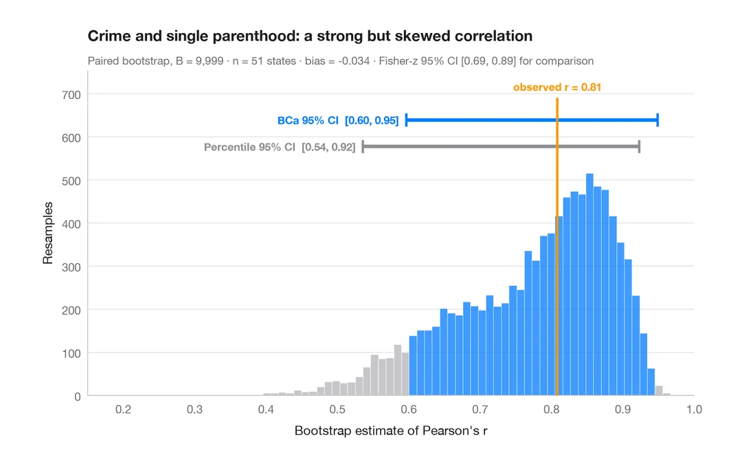
ブートストラップ分布
再標本化した相関係数を、パーセンタイル法と BCa 法の 95% 信頼区間とともに示します。
boot::boot() + boot::boot.ci()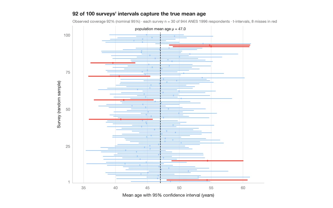
95% 信頼区間の意味
ANES の回答者 944 人から 30 人を抽出する調査を 100 回。平均年齢の 95% 信頼区間のうち真値を外したものを赤で示します。
teaching classic (e.g. TeachingDemos::ci.examp())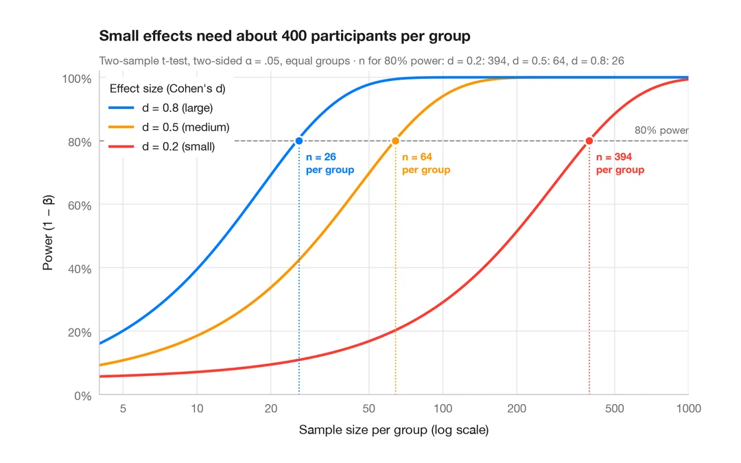
検出力曲線
2標本 t 検定の検出力を、小・中・大の効果量ごとに標本サイズに対して描きます。
pwr::pwr.t.test() + plot()