Silhouette plot for k-means
Do US states fall into distinct social profiles? k-means clusters next to their silhouette widths.
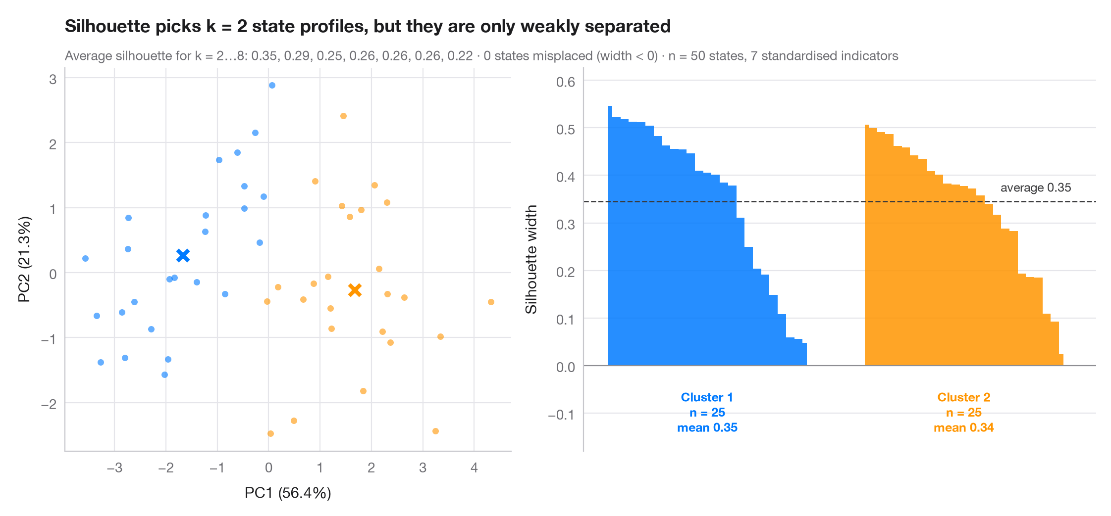
The silhouette width compares how close each observation is to its own cluster with how close it is to the nearest other cluster: near 1 means well placed, near 0 means on the border, negative means probably misassigned. The number of clusters k is the one with the highest average silhouette (2 to 8 tried). The left panel shows the clusters on the first two principal components; the right panel sorts the silhouette widths within each cluster, with the dashed line at the overall average.
Data are the 50 US states from the statsmodels statecrime dataset (2009
figures), described by 7 standardised indicators: violent-crime and murder
rates, % high-school graduates, % in poverty, % single-parent households,
% white and % urban. The District of Columbia is left out: it is so extreme
that k-means would give it a cluster of its own. The two clusters found are
roughly a lower-crime, lower-poverty profile and a higher-crime,
higher-poverty one, but an average silhouette around 0.35 is a weak
structure by Kaufman & Rousseeuw's rule of thumb (0.26–0.50): states form a
continuum more than separate types. KMeans, silhouette_score and
silhouette_samples from sklearn do the work; PCA is only used to draw
the clusters.
import matplotlib.pyplot as plt
import numpy as np
import statsmodels.api as sm
from sklearn.cluster import KMeans
from sklearn.decomposition import PCA
from sklearn.metrics import silhouette_samples, silhouette_score
from sklearn.preprocessing import StandardScaler

# 7 social indicators of the 50 US states (DC, an extreme outlier, is left out)
df = sm.datasets.statecrime.load_pandas().data.drop("District of Columbia")
X = StandardScaler().fit_transform(df)

# Choose k by the average silhouette width
fits = {k: KMeans(k, n_init=20, random_state=1).fit(X) for k in range(2, 9)}
avg = {k: silhouette_score(X, m.labels_) for k, m in fits.items()}
k = max(avg, key=avg.get)
labels = fits[k].labels_
sil = silhouette_samples(X, labels)
colors = ["#007AFF", "#FF9500", "#34C759", "#FF3B30", "#AF52DE", "#5AC8FA", "#8E8E93", "#A2845E"]

fig, (ax1, ax2) = plt.subplots(1, 2, figsize=(11, 5), width_ratios=[1, 1.15])

# Left: clusters projected on the first two principal components
pca = PCA(2).fit(X)
S, C = pca.transform(X), pca.transform(fits[k].cluster_centers_)
for j in range(k):
    ax1.scatter(*S[labels == j].T, s=22, color=colors[j], alpha=0.6, lw=0)
    ax1.scatter(*C[j], s=150, marker="X", color=colors[j], edgecolor="white", lw=1.5, zorder=3)
ax1.set_xlabel(f"PC1 ({100 * pca.explained_variance_ratio_[0]:.1f}%)")
ax1.set_ylabel(f"PC2 ({100 * pca.explained_variance_ratio_[1]:.1f}%)")
ax1.grid(axis="x")

# Right: silhouette widths, sorted within cluster
start = 0
for j in range(k):
    s = np.sort(sil[labels == j])[::-1]
    x = np.arange(start, start + len(s))
    ax2.fill_between(x, 0, s, color=colors[j], step="mid", lw=0, alpha=0.85)
    ax2.text(x.mean(), -0.05, f"Cluster {j + 1}\nn = {len(s)}\nmean {s.mean():.2f}",
             ha="center", va="top", fontsize=9, color=colors[j], fontweight="semibold")
    start += len(s) + 6
ax2.axhline(avg[k], color="#3A3A3C", ls="--", lw=1)
ax2.text(start - 6, avg[k] + 0.015, f"average {avg[k]:.2f}", ha="right", va="bottom",
         fontsize=9, color="#3A3A3C")
ax2.axhline(0, color="#8E8E93", lw=0.8)
ax2.set_xticks([])
ax2.set_xlim(-3, start - 3)
ax2.set_ylim(-0.18, max(sil) + 0.08)
ax2.set_ylabel("Silhouette width")
ax2.spines["bottom"].set_visible(False)

ax1.set_title(f"Silhouette picks k = {k} state profiles, but they are only weakly separated",
              pad=26)
ax1.text(0, 1.02, "Average silhouette for k = 2…8: " + ", ".join(f"{v:.2f}" for v in avg.values())
         + f" · {(sil < 0).sum()} states misplaced (width < 0) · n = {len(X)} states, "
         f"{X.shape[1]} standardised indicators", transform=ax1.transAxes, fontsize=9.5,
         color="#6E6E73", in_layout=False)
plt.show()
Figures use the optional PyStatlas style: add plt.style.use("pystatlas.mplstyle") to match the look exactly.
Data source
- US state crime and social indicators, 2009. U.S. Census Bureau. Statistical Abstract of the United States, state tables for 2009 (crime rates from the FBI Uniform Crime Reporting program). https://www.statsmodels.org/stable/datasets/generated/statecrime.html
Compiled for statsmodels (sm.datasets.statecrime); public domain. See the statsmodels page for each variable's table and footnotes.
The examples illustrate statistical methods. Their titles describe what each figure shows in these particular data — often a small, dated or partial sample — not the author's position on the substantive question. For interpretation, context and data quality, rely on the original sources cited here.
How to cite
PyStatlas is created and maintained by Thierry Warin. If it helped your work, please cite it.
Warin, T. (2026). Silhouette plot for k-means. In PyStatlas: A Python Gallery of Statistical Graphics for the Social Sciences. https://warint.github.io/pystatlas/multivariate/silhouette-clusters/
@misc{warin2026statlas,
  author       = {Warin, Thierry},
  title        = {PyStatlas: A Python Gallery of Statistical Graphics for the Social Sciences},
  year         = {2026},
  howpublished = {\url{https://warint.github.io/pystatlas/}},
  note         = {Source code: https://github.com/warint/pystatlas}
}More in Multivariate & clustering
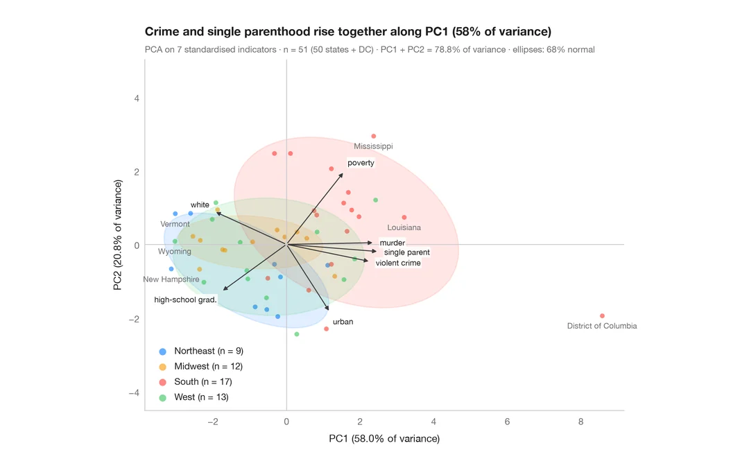
PCA biplot
US states and their social indicators on the first two principal components.
factoextra::fviz_pca_biplot()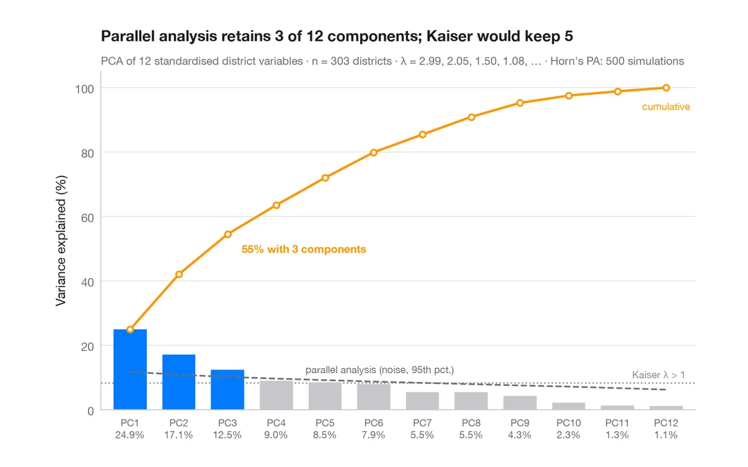
Scree plot
How many dimensions describe 303 California school districts? Variance per component and a parallel-analysis cut-off.
factoextra::fviz_eig()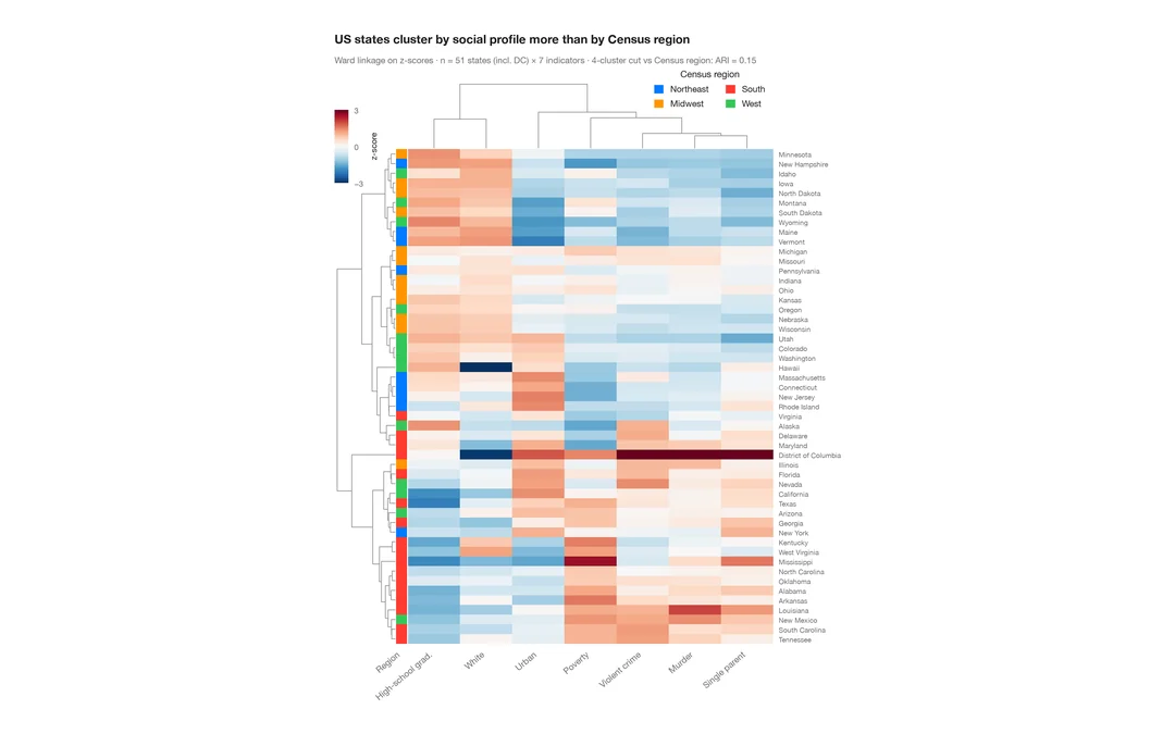
Clustered heatmap
Z-scored heatmap of US states' social indicators, with row and column dendrograms and a Census-region colour bar.
pheatmap::pheatmap() / ComplexHeatmap::Heatmap()