Scree plot
How many dimensions describe 303 California school districts? Variance per component and a parallel-analysis cut-off.
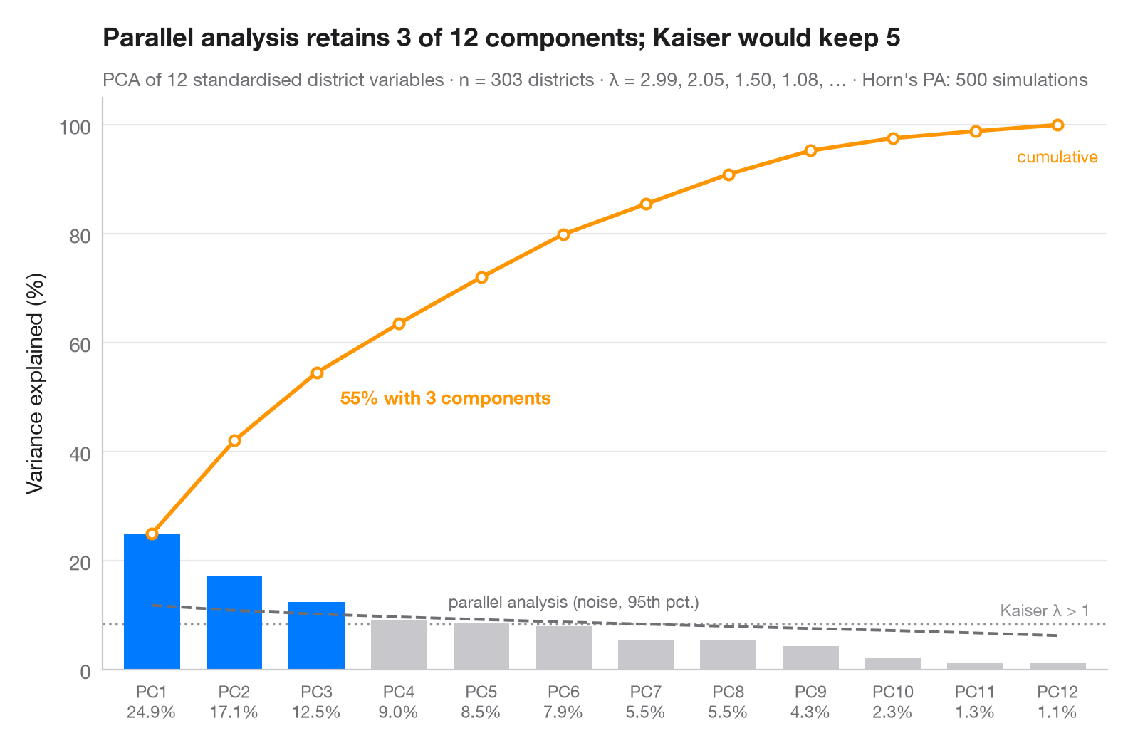
How many principal components are worth keeping? Bars show the share of variance carried by each component, the orange line the running total. The grey dashed line is Horn's parallel analysis: the 95th percentile of the same eigenvalues computed on random, uncorrelated data of the same size. A component is retained (blue) only if it beats that noise floor; the dotted line marks the older Kaiser rule (eigenvalue > 1).
Data are 303 California school districts from the statsmodels star98
dataset (1998 Standardized Testing and Reporting programme): 12 district
characteristics — % low-income pupils, % Asian, Black and Hispanic pupils,
% minority teachers, teachers' average experience and salary, per-pupil
spending, pupil–teacher ratio, % taking college-prep courses, % charter and
% year-round schools — each standardised. Eigenvalues of the correlation
matrix (the PCA variances) come from numpy.linalg.eigvalsh; the parallel
analysis is 500 seeded simulations. Note that parallel analysis keeps fewer
components than the Kaiser rule here.
import matplotlib.pyplot as plt
import numpy as np
import statsmodels.api as sm
from sklearn.preprocessing import StandardScaler

# PCA on 12 standardised characteristics of California school districts
X = StandardScaler().fit_transform(sm.datasets.star98.load_pandas().data.loc[:, "LOWINC":"PCTYRRND"])
n, p = X.shape
eig = np.sort(np.linalg.eigvalsh(np.corrcoef(X.T)))[::-1]  # PCA eigenvalues
pct = 100 * eig / eig.sum()

# Horn's parallel analysis: eigenvalues of pure noise, 95th percentile
rng = np.random.default_rng(42)
sims = [np.sort(np.linalg.eigvalsh(np.corrcoef(rng.normal(size=(n, p)).T)))[::-1]
        for _ in range(500)]
pa = np.percentile(sims, 95, axis=0)
keep = eig > pa
k = np.arange(1, p + 1)

fig, ax = plt.subplots(figsize=(8, 5))
ax.bar(k, pct, width=0.68, color=np.where(keep, "#007AFF", "#C7C7CC"), zorder=2)

# Cumulative share, parallel-analysis floor and Kaiser threshold (all in % of variance)
cum = np.cumsum(pct)
ax.plot(k, cum, color="#FF9500", marker="o", ms=5, mfc="white", mew=1.5, zorder=3)
ax.annotate(f"{cum[keep.sum() - 1]:.0f}% with {keep.sum()} components",
            (keep.sum(), cum[keep.sum() - 1]), xytext=(12, -16), textcoords="offset points",
            fontsize=9.5, color="#FF9500", fontweight="semibold")
ax.text(p, cum[-1] - 4, "cumulative", fontsize=8.5, color="#FF9500", ha="center", va="top")
ax.plot(k, 100 * pa / p, color="#6E6E73", ls="--", lw=1.4, zorder=3)
ax.text(4.6, 100 * pa[4] / p + 1.5, "parallel analysis (noise, 95th pct.)", fontsize=8.5,
        color="#6E6E73", va="bottom")
ax.axhline(100 / p, color="#8E8E93", ls=":", lw=1.2, zorder=1)
ax.text(p + 0.4, 100 / p + 0.8, "Kaiser λ > 1", fontsize=8.5, color="#8E8E93", ha="right", va="bottom")

ax.set_xticks(k, [f"PC{i}\n{v:.1f}%" for i, v in zip(k, pct)], fontsize=8.5)
ax.set_xlim(0.4, p + 0.6)
ax.set_ylim(0, 105)
ax.set_ylabel("Variance explained (%)")
ax.set_title(f"Parallel analysis retains {keep.sum()} of {p} components; Kaiser would keep "
             f"{(eig > 1).sum()}", pad=26)
ax.text(0, 1.02, f"PCA of {p} standardised district variables · n = {n} districts · λ = "
        f"{', '.join(f'{e:.2f}' for e in eig[:4])}, … · Horn's PA: 500 simulations",
        transform=ax.transAxes, fontsize=9.5, color="#6E6E73")
plt.show()
Figures use the optional PyStatlas style: add plt.style.use("pystatlas.mplstyle") to match the look exactly.
Data source
- California STAR test results, 1998 (303 school districts). Gill, J. (2001). Generalized Linear Models: A Unified Approach (Quantitative Applications in the Social Sciences, No. 134). Sage. https://www.statsmodels.org/stable/datasets/generated/star98.html
Original data from the California Department of Education's Standardized Testing and Reporting (STAR) program, 1998. Subset distributed with statsmodels (sm.datasets.star98) with the author's permission.
The examples illustrate statistical methods. Their titles describe what each figure shows in these particular data — often a small, dated or partial sample — not the author's position on the substantive question. For interpretation, context and data quality, rely on the original sources cited here.
How to cite
PyStatlas is created and maintained by Thierry Warin. If it helped your work, please cite it.
Warin, T. (2026). Scree plot. In PyStatlas: A Python Gallery of Statistical Graphics for the Social Sciences. https://warint.github.io/pystatlas/multivariate/scree-plot/
@misc{warin2026statlas,
  author       = {Warin, Thierry},
  title        = {PyStatlas: A Python Gallery of Statistical Graphics for the Social Sciences},
  year         = {2026},
  howpublished = {\url{https://warint.github.io/pystatlas/}},
  note         = {Source code: https://github.com/warint/pystatlas}
}More in Multivariate & clustering
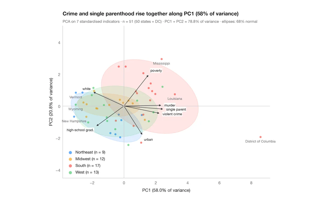
PCA biplot
US states and their social indicators on the first two principal components.
factoextra::fviz_pca_biplot()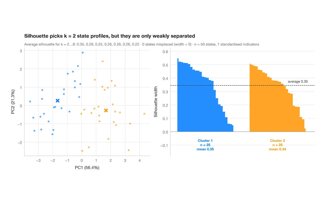
Silhouette plot for k-means
Do US states fall into distinct social profiles? k-means clusters next to their silhouette widths.
factoextra::fviz_silhouette()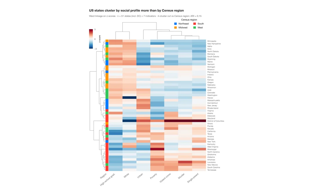
Clustered heatmap
Z-scored heatmap of US states' social indicators, with row and column dendrograms and a Census-region colour bar.
pheatmap::pheatmap() / ComplexHeatmap::Heatmap()