Clustered heatmap
Z-scored heatmap of US states' social indicators, with row and column dendrograms and a Census-region colour bar.
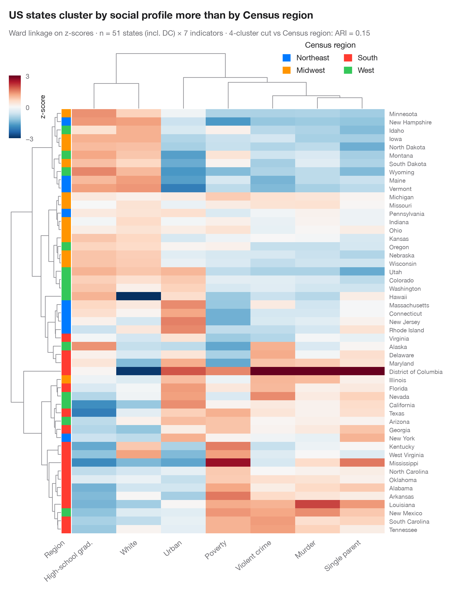
Each row is an observation, each column a variable, and each cell its z-score (blue below the variable's mean, red above). Rows and columns are reordered by hierarchical clustering (Ward linkage on Euclidean distance) and the dendrograms show the merge history. The colour bar on the left gives the known group of each row, so you can see at a glance whether the unsupervised tree rediscovers it — and which variables drive the split.
Data are the 50 US states and the District of Columbia from the statsmodels
statecrime dataset (2009 figures): violent-crime and murder rates per
100,000, % high-school graduates, % in poverty, % single-parent households,
% white and % urban population. The colour bar is the US Census region.
seaborn.clustermap does the clustering and drawing;
scipy.cluster.hierarchy cuts the row tree into four clusters to compute
the adjusted Rand index against the four regions: geography only partly
explains which states look alike.
import matplotlib.pyplot as plt
import numpy as np
import pandas as pd
import seaborn as sns
from matplotlib.patches import Patch
from scipy.cluster.hierarchy import fcluster
import statsmodels.api as sm
from sklearn.metrics import adjusted_rand_score

# Data: 7 social indicators of 51 US states (incl. DC), z-scored per column;
# US Census region as row annotation
df = sm.datasets.statecrime.load_pandas().data
df.index = df.index.str.strip()
Z = (df - df.mean()) / df.std()
Z.columns = ["Violent crime", "Murder", "High-school grad.", "Poverty", "Single parent",
             "White", "Urban"]
regions = {"Northeast": ["Connecticut", "Maine", "Massachusetts", "New Hampshire", "New Jersey",
                         "New York", "Pennsylvania", "Rhode Island", "Vermont"],
           "Midwest": ["Illinois", "Indiana", "Iowa", "Kansas", "Michigan", "Minnesota", "Missouri",
                       "Nebraska", "North Dakota", "Ohio", "South Dakota", "Wisconsin"],
           "West": ["Alaska", "Arizona", "California", "Colorado", "Hawaii", "Idaho", "Montana",
                    "Nevada", "New Mexico", "Oregon", "Utah", "Washington", "Wyoming"]}
region = pd.Series([next((r for r, s in regions.items() if st in s), "South") for st in Z.index],
                   index=Z.index, name="Region")
palette = dict(zip(["Northeast", "Midwest", "South", "West"],
                   ["#007AFF", "#FF9500", "#FF3B30", "#34C759"]))

with plt.rc_context({"figure.constrained_layout.use": False}):
    g = sns.clustermap(Z, method="ward", metric="euclidean", cmap="RdBu_r", center=0,
                       vmin=-3, vmax=3, row_colors=region.map(palette), yticklabels=True,
                       figsize=(8.5, 10), dendrogram_ratio=(0.14, 0.12), colors_ratio=0.025,
                       cbar_pos=(0.02, 0.83, 0.025, 0.11),
                       cbar_kws=dict(label="z-score", ticks=[-3, 0, 3]),
                       tree_kws=dict(colors="#8E8E93", linewidths=0.8))

# How well does the row tree, cut into four clusters, recover the Census regions?
ari = adjusted_rand_score(region, fcluster(g.dendrogram_row.linkage, 4, "maxclust"))

g.ax_heatmap.set_xticklabels(g.ax_heatmap.get_xticklabels(), rotation=40, ha="right", fontsize=9.5)
g.ax_heatmap.set(xlabel="", ylabel="")
g.ax_heatmap.tick_params(axis="y", length=0, labelsize=7.5)
g.ax_heatmap.tick_params(axis="x", length=0)
g.ax_row_colors.set_xticklabels(["Region"], rotation=40, ha="right", fontsize=9.5)
g.ax_row_colors.tick_params(axis="x", length=0)
g.ax_cbar.tick_params(labelsize=8.5)
g.ax_cbar.yaxis.label.set_size(9)
g.ax_col_dendrogram.legend(handles=[Patch(color=c, label=n) for n, c in palette.items()],
                           loc="upper right", bbox_to_anchor=(1.0, 1.3), fontsize=9.5, ncol=2,
                           title="Census region", frameon=False, handlelength=1, handleheight=1)

g.figure.text(0.02, 1.04, "US states cluster by social profile more than by Census region",
              fontsize=13, fontweight="semibold", color="#1D1D1F")
g.figure.text(0.02, 1.01, f"Ward linkage on z-scores · n = {len(Z)} states (incl. DC) × {Z.shape[1]} "
              f"indicators · 4-cluster cut vs Census region: ARI = {ari:.2f}",
              fontsize=9.5, color="#6E6E73")
plt.show()
Figures use the optional PyStatlas style: add plt.style.use("pystatlas.mplstyle") to match the look exactly.
Data source
- US state crime and social indicators, 2009. U.S. Census Bureau. Statistical Abstract of the United States, state tables for 2009 (crime rates from the FBI Uniform Crime Reporting program). https://www.statsmodels.org/stable/datasets/generated/statecrime.html
Compiled for statsmodels (sm.datasets.statecrime); public domain. See the statsmodels page for each variable's table and footnotes.
The examples illustrate statistical methods. Their titles describe what each figure shows in these particular data — often a small, dated or partial sample — not the author's position on the substantive question. For interpretation, context and data quality, rely on the original sources cited here.
How to cite
PyStatlas is created and maintained by Thierry Warin. If it helped your work, please cite it.
Warin, T. (2026). Clustered heatmap. In PyStatlas: A Python Gallery of Statistical Graphics for the Social Sciences. https://warint.github.io/pystatlas/multivariate/clustered-heatmap/
@misc{warin2026statlas,
  author       = {Warin, Thierry},
  title        = {PyStatlas: A Python Gallery of Statistical Graphics for the Social Sciences},
  year         = {2026},
  howpublished = {\url{https://warint.github.io/pystatlas/}},
  note         = {Source code: https://github.com/warint/pystatlas}
}More in Multivariate & clustering
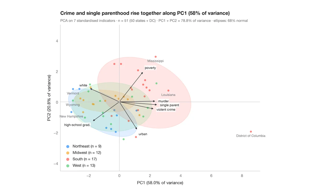
PCA biplot
US states and their social indicators on the first two principal components.
factoextra::fviz_pca_biplot()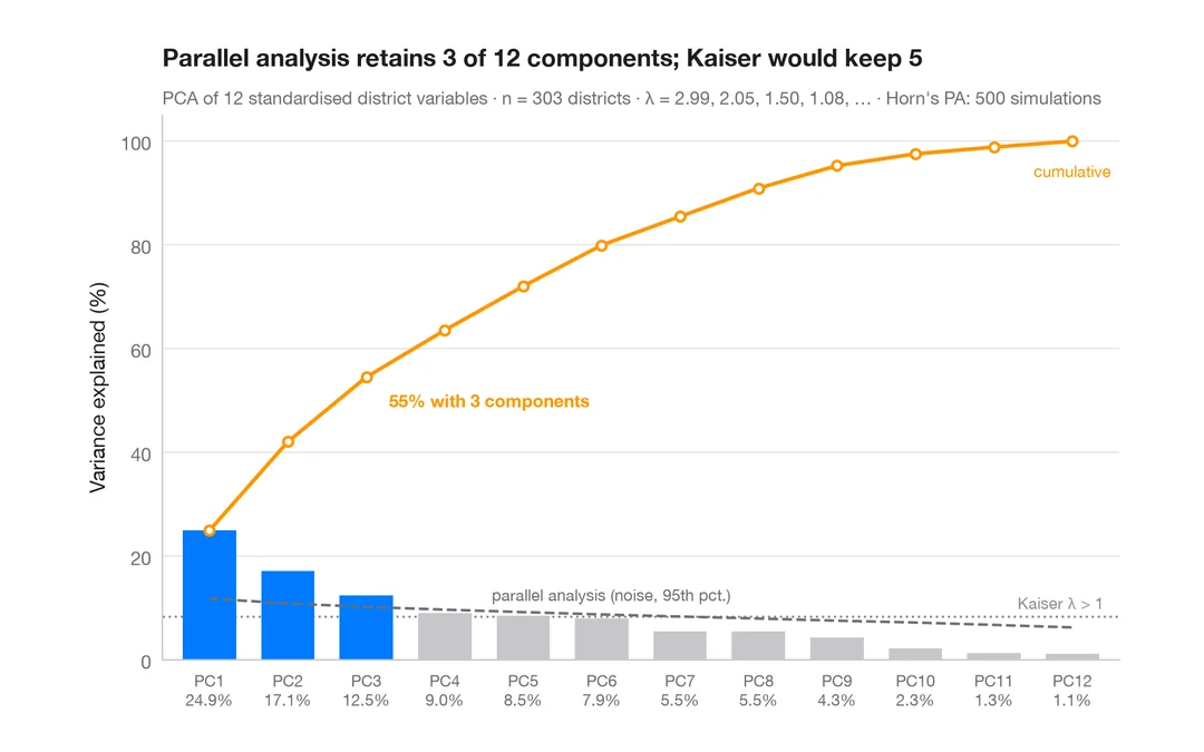
Scree plot
How many dimensions describe 303 California school districts? Variance per component and a parallel-analysis cut-off.
factoextra::fviz_eig()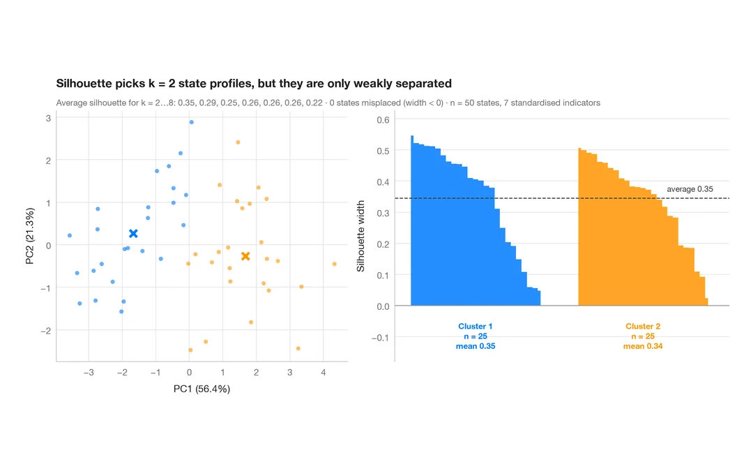
Silhouette plot for k-means
Do US states fall into distinct social profiles? k-means clusters next to their silhouette widths.
factoextra::fviz_silhouette()