聚类热图
美国各州社会指标的 z 分数热图,带行列树状图和人口普查区域色条。
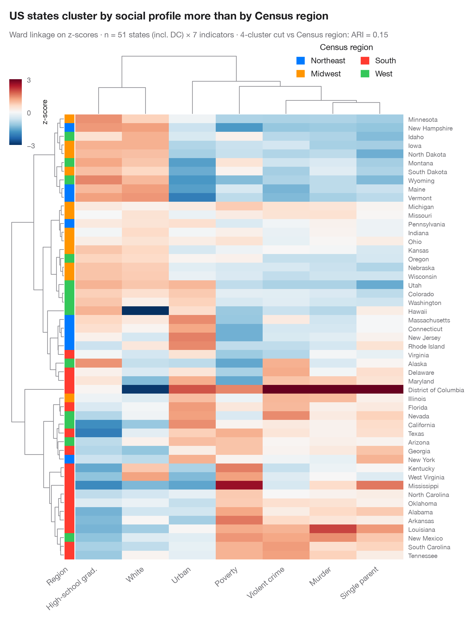
每一行是一个观测,每一列是一个变量,每个单元格是其 z 分数(低于该变量均值为蓝色,高于为红色)。行和列按层次聚类(基于欧氏距离的 Ward 连接法)重新排序,树状图展示合并过程。左侧色条给出每一行的已知分组,一眼就能看出无监督的聚类树是否重新发现了它——以及哪些变量主导了划分。
数据为 statsmodels statecrime 数据集中的美国 50 个州和哥伦比亚特区(2009 年数据):每 10 万人暴力犯罪率和谋杀率、高中毕业生比例、贫困人口比例、单亲家庭比例、白人比例和城市人口比例。色条为美国人口普查局的区域划分。seaborn.clustermap 完成聚类和绘图;scipy.cluster.hierarchy 将行聚类树切成四个簇,计算其与四个区域之间的调整兰德指数:地理位置只能部分解释哪些州彼此相似。
代码及图中文字均为英文。
import matplotlib.pyplot as plt
import numpy as np
import pandas as pd
import seaborn as sns
from matplotlib.patches import Patch
from scipy.cluster.hierarchy import fcluster
import statsmodels.api as sm
from sklearn.metrics import adjusted_rand_score

# Data: 7 social indicators of 51 US states (incl. DC), z-scored per column;
# US Census region as row annotation
df = sm.datasets.statecrime.load_pandas().data
df.index = df.index.str.strip()
Z = (df - df.mean()) / df.std()
Z.columns = ["Violent crime", "Murder", "High-school grad.", "Poverty", "Single parent",
             "White", "Urban"]
regions = {"Northeast": ["Connecticut", "Maine", "Massachusetts", "New Hampshire", "New Jersey",
                         "New York", "Pennsylvania", "Rhode Island", "Vermont"],
           "Midwest": ["Illinois", "Indiana", "Iowa", "Kansas", "Michigan", "Minnesota", "Missouri",
                       "Nebraska", "North Dakota", "Ohio", "South Dakota", "Wisconsin"],
           "West": ["Alaska", "Arizona", "California", "Colorado", "Hawaii", "Idaho", "Montana",
                    "Nevada", "New Mexico", "Oregon", "Utah", "Washington", "Wyoming"]}
region = pd.Series([next((r for r, s in regions.items() if st in s), "South") for st in Z.index],
                   index=Z.index, name="Region")
palette = dict(zip(["Northeast", "Midwest", "South", "West"],
                   ["#007AFF", "#FF9500", "#FF3B30", "#34C759"]))

with plt.rc_context({"figure.constrained_layout.use": False}):
    g = sns.clustermap(Z, method="ward", metric="euclidean", cmap="RdBu_r", center=0,
                       vmin=-3, vmax=3, row_colors=region.map(palette), yticklabels=True,
                       figsize=(8.5, 10), dendrogram_ratio=(0.14, 0.12), colors_ratio=0.025,
                       cbar_pos=(0.02, 0.83, 0.025, 0.11),
                       cbar_kws=dict(label="z-score", ticks=[-3, 0, 3]),
                       tree_kws=dict(colors="#8E8E93", linewidths=0.8))

# How well does the row tree, cut into four clusters, recover the Census regions?
ari = adjusted_rand_score(region, fcluster(g.dendrogram_row.linkage, 4, "maxclust"))

g.ax_heatmap.set_xticklabels(g.ax_heatmap.get_xticklabels(), rotation=40, ha="right", fontsize=9.5)
g.ax_heatmap.set(xlabel="", ylabel="")
g.ax_heatmap.tick_params(axis="y", length=0, labelsize=7.5)
g.ax_heatmap.tick_params(axis="x", length=0)
g.ax_row_colors.set_xticklabels(["Region"], rotation=40, ha="right", fontsize=9.5)
g.ax_row_colors.tick_params(axis="x", length=0)
g.ax_cbar.tick_params(labelsize=8.5)
g.ax_cbar.yaxis.label.set_size(9)
g.ax_col_dendrogram.legend(handles=[Patch(color=c, label=n) for n, c in palette.items()],
                           loc="upper right", bbox_to_anchor=(1.0, 1.3), fontsize=9.5, ncol=2,
                           title="Census region", frameon=False, handlelength=1, handleheight=1)

g.figure.text(0.02, 1.04, "US states cluster by social profile more than by Census region",
              fontsize=13, fontweight="semibold", color="#1D1D1F")
g.figure.text(0.02, 1.01, f"Ward linkage on z-scores · n = {len(Z)} states (incl. DC) × {Z.shape[1]} "
              f"indicators · 4-cluster cut vs Census region: ARI = {ari:.2f}",
              fontsize=9.5, color="#6E6E73")
plt.show()
图表使用了可选的 PyStatlas 样式:添加 plt.style.use("pystatlas.mplstyle") 即可完全还原其外观。
数据来源
- US state crime and social indicators, 2009. U.S. Census Bureau. Statistical Abstract of the United States, state tables for 2009 (crime rates from the FBI Uniform Crime Reporting program). https://www.statsmodels.org/stable/datasets/generated/statecrime.html
Compiled for statsmodels (sm.datasets.statecrime); public domain. See the statsmodels page for each variable's table and footnotes.
这些示例用于说明统计方法。图表标题描述的是该图在这些特定数据中呈现的内容——这些数据往往样本较小、年代较早或并不完整——而不是作者对实质问题的立场。关于解释、背景和数据质量,请以此处引用的原始来源为准。
如何引用
PyStatlas 由 Thierry Warin 创建并维护。如果它对你的工作有所帮助,敬请引用。
Warin, T. (2026). Clustered heatmap. In PyStatlas: A Python Gallery of Statistical Graphics for the Social Sciences. https://warint.github.io/pystatlas/multivariate/clustered-heatmap/
@misc{warin2026statlas,
  author       = {Warin, Thierry},
  title        = {PyStatlas: A Python Gallery of Statistical Graphics for the Social Sciences},
  year         = {2026},
  howpublished = {\url{https://warint.github.io/pystatlas/}},
  note         = {Source code: https://github.com/warint/pystatlas}
}