碎石图
描述加州 303 个学区需要几个维度?各主成分的方差及平行分析截断值。
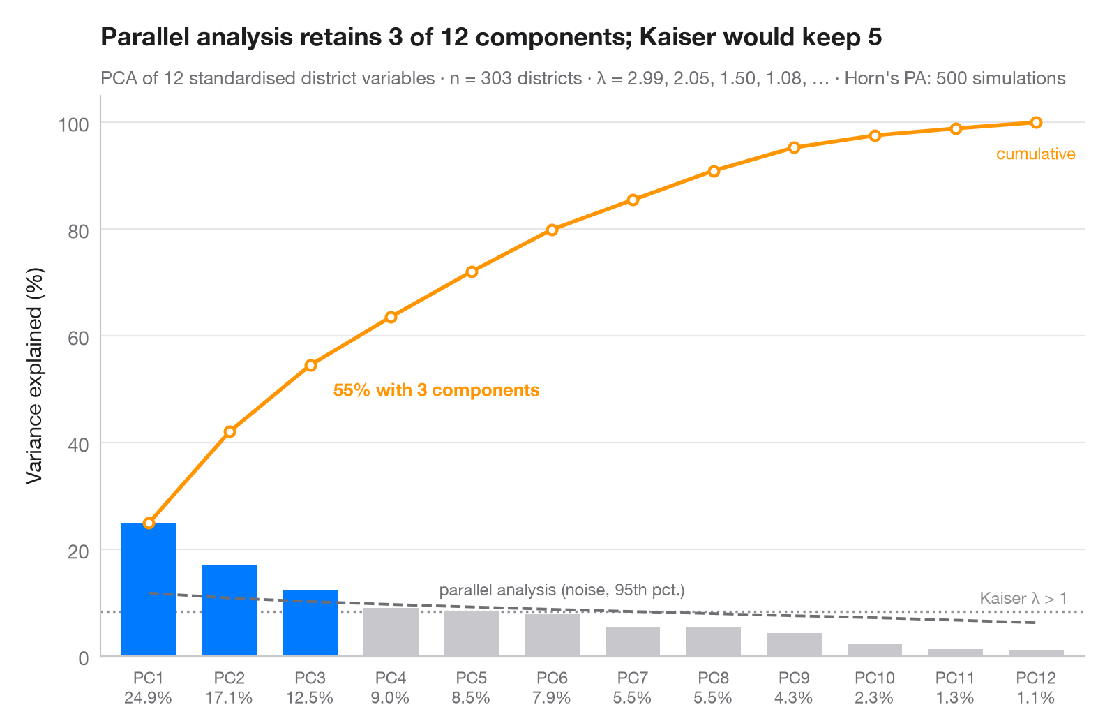
值得保留多少个主成分?柱形表示每个主成分承载的方差占比,橙色线为累计占比。灰色虚线是 Horn 平行分析:在同样规模、互不相关的随机数据上计算出的特征值的第 95 百分位数。只有超过这一噪声下限的主成分才会被保留(蓝色);点线标出较早的 Kaiser 准则(特征值 > 1)。
数据为 statsmodels star98 数据集中的 303 个加州学区(1998 年 Standardized Testing and Reporting 项目):12 项学区特征——低收入学生比例,亚裔、黑人和西班牙裔学生比例,少数族裔教师比例,教师平均教龄和平均薪资,生均支出,生师比,修读大学预备课程的学生比例,特许学校比例和全年制学校比例——均经过标准化。相关矩阵的特征值(即 PCA 方差)由 numpy.linalg.eigvalsh 计算;平行分析为 500 次固定种子的模拟。注意,此处平行分析保留的主成分少于 Kaiser 准则。
代码及图中文字均为英文。
import matplotlib.pyplot as plt
import numpy as np
import statsmodels.api as sm
from sklearn.preprocessing import StandardScaler

# PCA on 12 standardised characteristics of California school districts
X = StandardScaler().fit_transform(sm.datasets.star98.load_pandas().data.loc[:, "LOWINC":"PCTYRRND"])
n, p = X.shape
eig = np.sort(np.linalg.eigvalsh(np.corrcoef(X.T)))[::-1]  # PCA eigenvalues
pct = 100 * eig / eig.sum()

# Horn's parallel analysis: eigenvalues of pure noise, 95th percentile
rng = np.random.default_rng(42)
sims = [np.sort(np.linalg.eigvalsh(np.corrcoef(rng.normal(size=(n, p)).T)))[::-1]
        for _ in range(500)]
pa = np.percentile(sims, 95, axis=0)
keep = eig > pa
k = np.arange(1, p + 1)

fig, ax = plt.subplots(figsize=(8, 5))
ax.bar(k, pct, width=0.68, color=np.where(keep, "#007AFF", "#C7C7CC"), zorder=2)

# Cumulative share, parallel-analysis floor and Kaiser threshold (all in % of variance)
cum = np.cumsum(pct)
ax.plot(k, cum, color="#FF9500", marker="o", ms=5, mfc="white", mew=1.5, zorder=3)
ax.annotate(f"{cum[keep.sum() - 1]:.0f}% with {keep.sum()} components",
            (keep.sum(), cum[keep.sum() - 1]), xytext=(12, -16), textcoords="offset points",
            fontsize=9.5, color="#FF9500", fontweight="semibold")
ax.text(p, cum[-1] - 4, "cumulative", fontsize=8.5, color="#FF9500", ha="center", va="top")
ax.plot(k, 100 * pa / p, color="#6E6E73", ls="--", lw=1.4, zorder=3)
ax.text(4.6, 100 * pa[4] / p + 1.5, "parallel analysis (noise, 95th pct.)", fontsize=8.5,
        color="#6E6E73", va="bottom")
ax.axhline(100 / p, color="#8E8E93", ls=":", lw=1.2, zorder=1)
ax.text(p + 0.4, 100 / p + 0.8, "Kaiser λ > 1", fontsize=8.5, color="#8E8E93", ha="right", va="bottom")

ax.set_xticks(k, [f"PC{i}\n{v:.1f}%" for i, v in zip(k, pct)], fontsize=8.5)
ax.set_xlim(0.4, p + 0.6)
ax.set_ylim(0, 105)
ax.set_ylabel("Variance explained (%)")
ax.set_title(f"Parallel analysis retains {keep.sum()} of {p} components; Kaiser would keep "
             f"{(eig > 1).sum()}", pad=26)
ax.text(0, 1.02, f"PCA of {p} standardised district variables · n = {n} districts · λ = "
        f"{', '.join(f'{e:.2f}' for e in eig[:4])}, … · Horn's PA: 500 simulations",
        transform=ax.transAxes, fontsize=9.5, color="#6E6E73")
plt.show()
图表使用了可选的 PyStatlas 样式:添加 plt.style.use("pystatlas.mplstyle") 即可完全还原其外观。
数据来源
- California STAR test results, 1998 (303 school districts). Gill, J. (2001). Generalized Linear Models: A Unified Approach (Quantitative Applications in the Social Sciences, No. 134). Sage. https://www.statsmodels.org/stable/datasets/generated/star98.html
Original data from the California Department of Education's Standardized Testing and Reporting (STAR) program, 1998. Subset distributed with statsmodels (sm.datasets.star98) with the author's permission.
这些示例用于说明统计方法。图表标题描述的是该图在这些特定数据中呈现的内容——这些数据往往样本较小、年代较早或并不完整——而不是作者对实质问题的立场。关于解释、背景和数据质量,请以此处引用的原始来源为准。
如何引用
PyStatlas 由 Thierry Warin 创建并维护。如果它对你的工作有所帮助,敬请引用。
Warin, T. (2026). Scree plot. In PyStatlas: A Python Gallery of Statistical Graphics for the Social Sciences. https://warint.github.io/pystatlas/multivariate/scree-plot/
@misc{warin2026statlas,
  author       = {Warin, Thierry},
  title        = {PyStatlas: A Python Gallery of Statistical Graphics for the Social Sciences},
  year         = {2026},
  howpublished = {\url{https://warint.github.io/pystatlas/}},
  note         = {Source code: https://github.com/warint/pystatlas}
}