Scree plot — PyStatlas: A Python Gallery of Statistical Graphics for the Social Sciences

Warin, Thierry

スクリープロット

カリフォルニア州の 303 学区を記述するには何次元が必要か？成分ごとの分散と平行分析による基準。

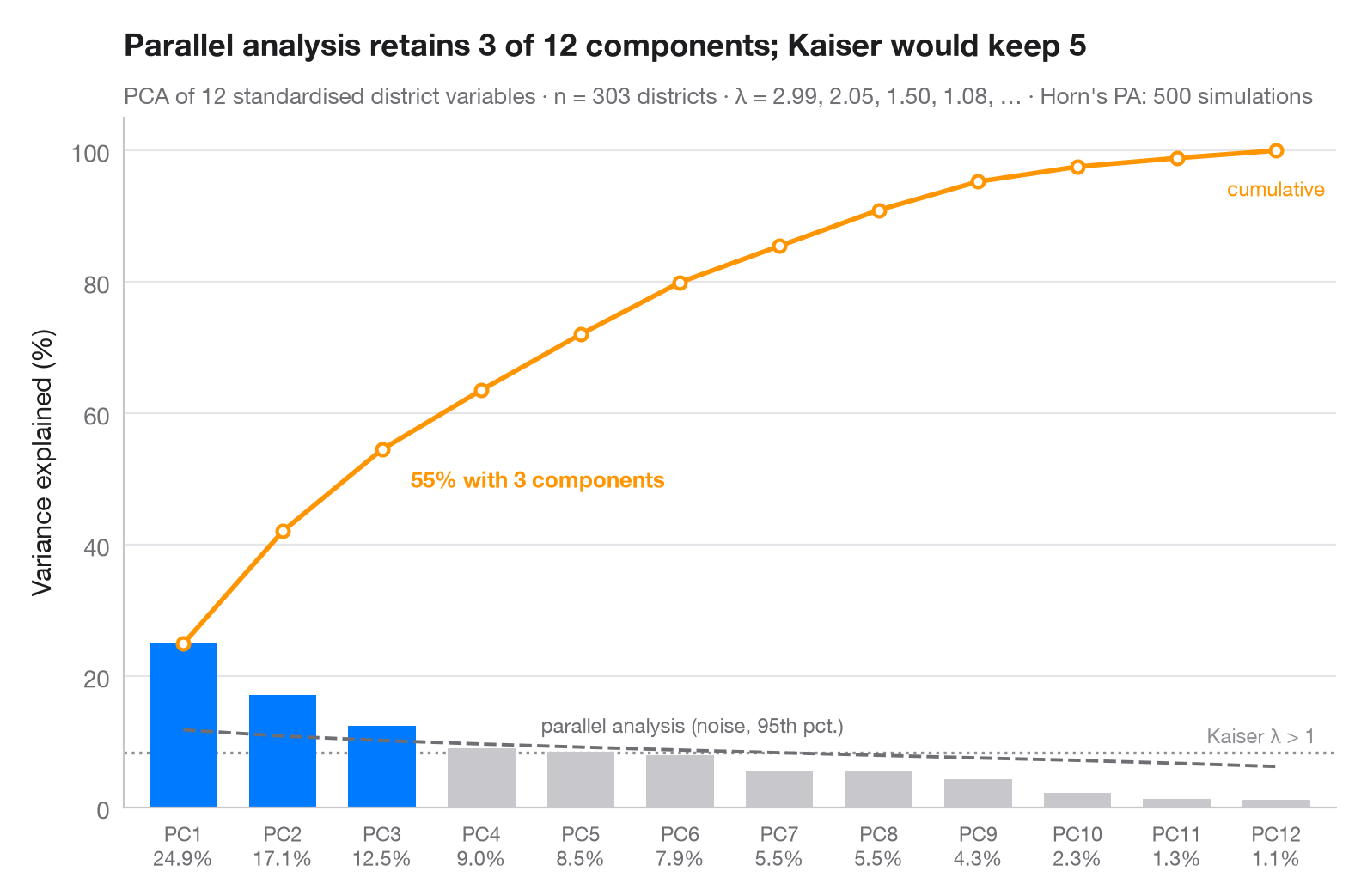
主成分はいくつ残す価値があるでしょうか。棒は各成分が担う分散の割合、オレンジの線はその累積です。灰色の破線はホーンの平行分析で、同じ大きさの無相関な乱数データから計算した固有値の 95 パーセンタイルです。成分はこのノイズの床を上回る場合にのみ保持され（青）、点線は従来のカイザー基準（固有値 > 1）を示します。

データは statsmodels の star98 データセット（1998 年の Standardized Testing and Reporting プログラム）に含まれるカリフォルニア州の 303 学区です。学区の 12 の特性 — 低所得家庭の児童生徒の割合、アジア系・黒人・ヒスパニック系の児童生徒の割合、マイノリティ教員の割合、教員の平均経験年数と平均給与、生徒 1 人あたり支出、生徒対教員比、大学進学準備科目の履修者の割合、チャータースクールの割合、通年制学校の割合 — をそれぞれ標準化しています。相関行列の固有値（PCA の分散）は numpy.linalg.eigvalsh で求め、平行分析はシードを固定した 500 回のシミュレーションです。ここでは平行分析がカイザー基準より少ない成分を残す点に注意してください。

コードおよび図中のテキストは英語です。

scree-plot.py · 45 行

ダウンロード GitHub

import matplotlib.pyplot as plt
import numpy as np
import statsmodels.api as sm
from sklearn.preprocessing import StandardScaler

# PCA on 12 standardised characteristics of California school districts
X = StandardScaler().fit_transform(sm.datasets.star98.load_pandas().data.loc[:, "LOWINC":"PCTYRRND"])
n, p = X.shape
eig = np.sort(np.linalg.eigvalsh(np.corrcoef(X.T)))[::-1]  # PCA eigenvalues
pct = 100 * eig / eig.sum()

# Horn's parallel analysis: eigenvalues of pure noise, 95th percentile
rng = np.random.default_rng(42)
sims = [np.sort(np.linalg.eigvalsh(np.corrcoef(rng.normal(size=(n, p)).T)))[::-1]
        for _ in range(500)]
pa = np.percentile(sims, 95, axis=0)
keep = eig > pa
k = np.arange(1, p + 1)

fig, ax = plt.subplots(figsize=(8, 5))
ax.bar(k, pct, width=0.68, color=np.where(keep, "#007AFF", "#C7C7CC"), zorder=2)

# Cumulative share, parallel-analysis floor and Kaiser threshold (all in % of variance)
cum = np.cumsum(pct)
ax.plot(k, cum, color="#FF9500", marker="o", ms=5, mfc="white", mew=1.5, zorder=3)
ax.annotate(f"{cum[keep.sum() - 1]:.0f}% with {keep.sum()} components",
            (keep.sum(), cum[keep.sum() - 1]), xytext=(12, -16), textcoords="offset points",
            fontsize=9.5, color="#FF9500", fontweight="semibold")
ax.text(p, cum[-1] - 4, "cumulative", fontsize=8.5, color="#FF9500", ha="center", va="top")
ax.plot(k, 100 * pa / p, color="#6E6E73", ls="--", lw=1.4, zorder=3)
ax.text(4.6, 100 * pa[4] / p + 1.5, "parallel analysis (noise, 95th pct.)", fontsize=8.5,
        color="#6E6E73", va="bottom")
ax.axhline(100 / p, color="#8E8E93", ls=":", lw=1.2, zorder=1)
ax.text(p + 0.4, 100 / p + 0.8, "Kaiser λ > 1", fontsize=8.5, color="#8E8E93", ha="right", va="bottom")

ax.set_xticks(k, [f"PC{i}\n{v:.1f}%" for i, v in zip(k, pct)], fontsize=8.5)
ax.set_xlim(0.4, p + 0.6)
ax.set_ylim(0, 105)
ax.set_ylabel("Variance explained (%)")
ax.set_title(f"Parallel analysis retains {keep.sum()} of {p} components; Kaiser would keep "
             f"{(eig > 1).sum()}", pad=26)
ax.text(0, 1.02, f"PCA of {p} standardised district variables · n = {n} districts · λ = "
        f"{', '.join(f'{e:.2f}' for e in eig[:4])}, … · Horn's PA: 500 simulations",
        transform=ax.transAxes, fontsize=9.5, color="#6E6E73")
plt.show()

図にはオプションの PyStatlas スタイルを使用しています。同じ見た目にするには plt.style.use("pystatlas.mplstyle") を追加してください。

データの出典

California STAR test results, 1998 (303 school districts). Gill, J. (2001). Generalized Linear Models: A Unified Approach (Quantitative Applications in the Social Sciences, No. 134). Sage. https://www.statsmodels.org/stable/datasets/generated/star98.html
Original data from the California Department of Education's Standardized Testing and Reporting (STAR) program, 1998. Subset distributed with statsmodels (sm.datasets.star98) with the author's permission.

これらの例は統計手法を説明するためのものです。図のタイトルは、この特定のデータ（多くは小規模で、古く、部分的な標本）で図が示す内容を述べたものであり、実質的な問いに対する著者の立場ではありません。解釈、背景、データの質については、ここに挙げた元の出典を参照してください。

引用方法

PyStatlas は Thierry Warin が作成・運営しています。研究や業務に役立った場合は、ぜひ引用してください。

Warin, T. (2026). Scree plot. In PyStatlas: A Python Gallery of Statistical Graphics for the Social Sciences. https://warint.github.io/pystatlas/multivariate/scree-plot/

@misc{warin2026statlas,
  author       = {Warin, Thierry},
  title        = {PyStatlas: A Python Gallery of Statistical Graphics for the Social Sciences},
  year         = {2026},
  howpublished = {\url{https://warint.github.io/pystatlas/}},
  note         = {Source code: https://github.com/warint/pystatlas}
}

多変量解析とクラスタリングのその他のグラフ

多変量解析とクラスタリング

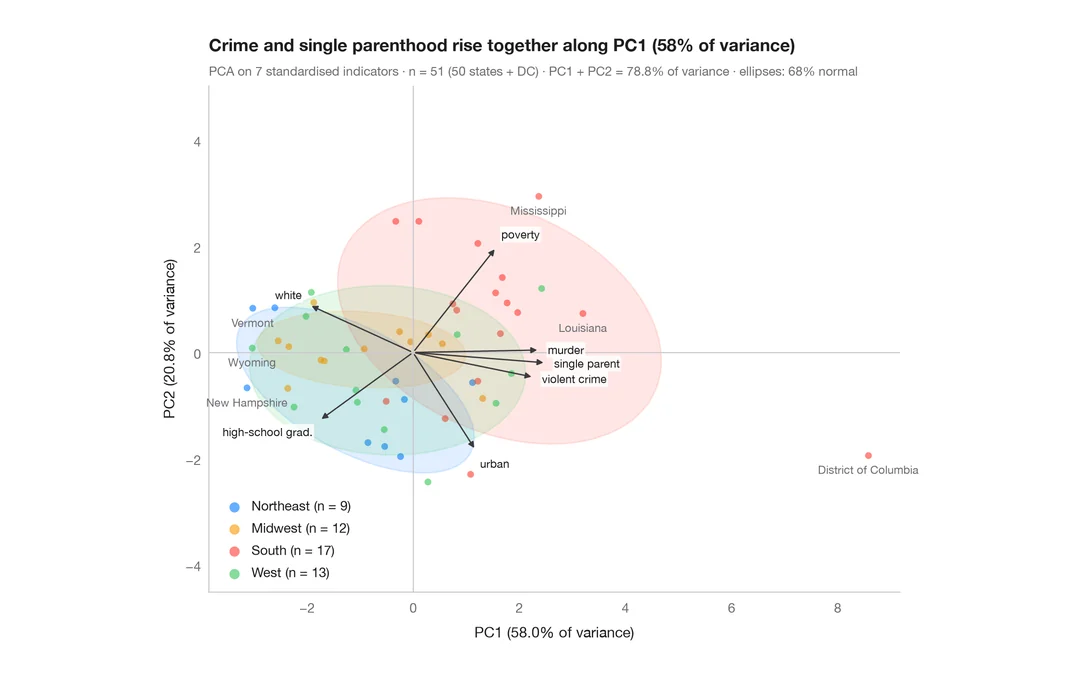
PCA バイプロット

米国の州とその社会指標を第 1・第 2 主成分の平面に配置します。

factoextra::fviz_pca_biplot()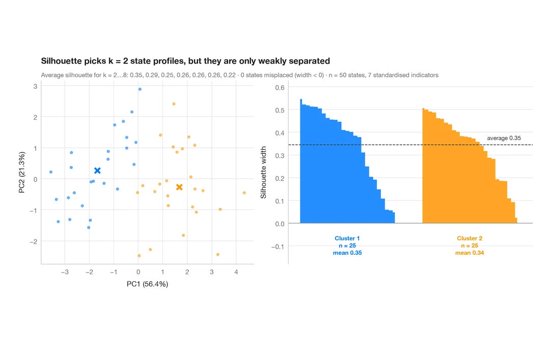

多変量解析とクラスタリング

k-means のシルエットプロット

米国の州ははっきり異なる社会的プロファイルに分かれるか？k-means のクラスターとシルエット幅。

factoextra::fviz_silhouette()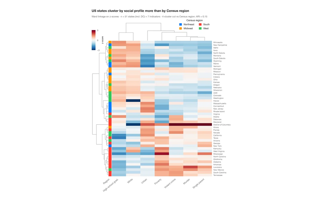

多変量解析とクラスタリング

クラスター化ヒートマップ

米国各州の社会指標の z スコアのヒートマップ。行と列のデンドログラム、国勢調査地域のカラーバー付き。

pheatmap::pheatmap() / ComplexHeatmap::Heatmap()