PCA バイプロット
米国の州とその社会指標を第 1・第 2 主成分の平面に配置します。
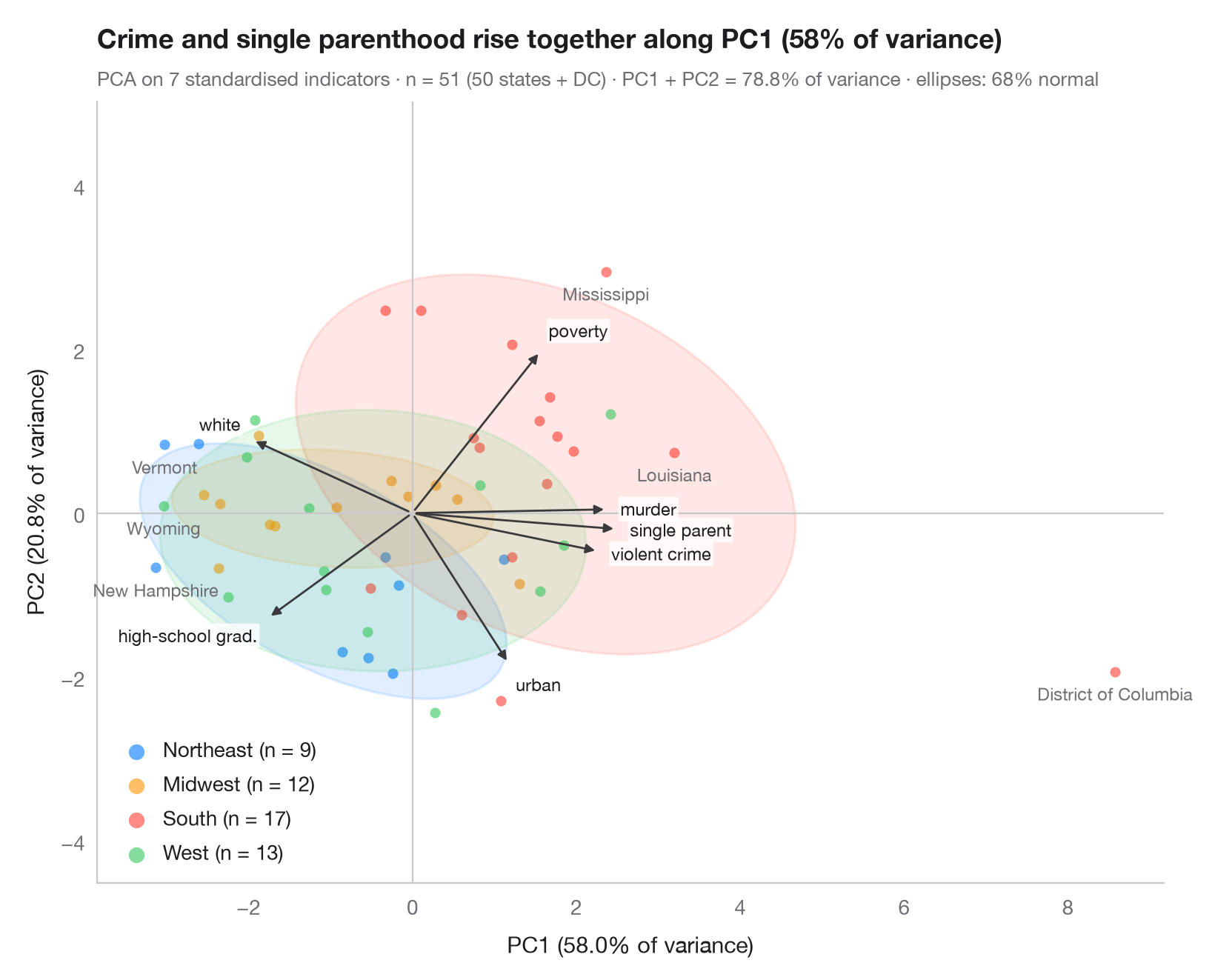
バイプロットは、同じ主成分平面に 2 つの要素を重ねて描きます。スコア(観測ごとに 1 点、グループ別に色分けし、グループごとに 68% の正規楕円を付与)と負荷量(変数ごとに 1 本の矢印)です。同じ方向を向く矢印どうしは正の相関があり、長い矢印は表示中の 2 成分に強く寄与します。各グループは、値が高い変数の側に位置します。
データは statsmodels の statecrime データセット(2009 年の数値)に含まれる米国 50 州とコロンビア特別区です。人口 10 万人あたりの暴力犯罪率と殺人率、高校卒業者の割合、貧困線以下の割合、ひとり親世帯の割合、白人の割合、都市人口の割合を用います。州は国勢調査局の地域区分で色分けし、最も極端な 6 州に名前を付けています。変数を標準化したうえで、sklearn.decomposition.PCA がスコア、負荷量、各軸に示す分散の割合を求めます。
コードおよび図中のテキストは英語です。
import matplotlib.pyplot as plt
import numpy as np
import statsmodels.api as sm
from matplotlib.patches import Ellipse
from scipy import stats
from sklearn.decomposition import PCA
from sklearn.preprocessing import StandardScaler

# Data: 7 social indicators of 51 US states (incl. DC), standardised
df = sm.datasets.statecrime.load_pandas().data
states = df.index.str.strip()
X = StandardScaler().fit_transform(df)
regions = {"Northeast": ["Connecticut", "Maine", "Massachusetts", "New Hampshire", "New Jersey",
                         "New York", "Pennsylvania", "Rhode Island", "Vermont"],
           "Midwest": ["Illinois", "Indiana", "Iowa", "Kansas", "Michigan", "Minnesota", "Missouri",
                       "Nebraska", "North Dakota", "Ohio", "South Dakota", "Wisconsin"],
           "West": ["Alaska", "Arizona", "California", "Colorado", "Hawaii", "Idaho", "Montana",
                    "Nevada", "New Mexico", "Oregon", "Utah", "Washington", "Wyoming"]}
groups = np.array([next((r for r, s in regions.items() if st in s), "South") for st in states])
names = ["violent crime", "murder", "high-school grad.", "poverty", "single parent",
         "white", "urban"]

pca = PCA(n_components=2).fit(X)
scores = pca.transform(X)
loadings = pca.components_.T * np.sqrt(pca.explained_variance_)  # variable–PC correlations
var = pca.explained_variance_ratio_ * 100

fig, ax = plt.subplots(figsize=(8, 6.4))
ax.axhline(0, color="#C7C7CC", lw=0.8); ax.axvline(0, color="#C7C7CC", lw=0.8)
r68 = np.sqrt(stats.chi2.ppf(0.68, df=2))
for g, c in zip(["Northeast", "Midwest", "South", "West"], ["#007AFF", "#FF9500", "#FF3B30", "#34C759"]):
    s = scores[groups == g]
    ax.scatter(*s.T, s=26, color=c, alpha=0.6, lw=0, label=f"{g} (n = {len(s)})")
    # 68% normal-theory ellipse from the group covariance
    vals, vecs = np.linalg.eigh(np.cov(s.T))
    angle = np.degrees(np.arctan2(vecs[1, 1], vecs[0, 1]))
    ax.add_patch(Ellipse(s.mean(0), *(2 * r68 * np.sqrt(vals[::-1])), angle=angle,
                         facecolor=c, alpha=0.12, edgecolor=c, lw=1.2))

# Name the six states farthest from the centre
for i in np.argsort(-np.hypot(*scores.T))[:6]:
    ax.annotate(states[i], scores[i], xytext=(0, -6), textcoords="offset points", fontsize=8.5,
                color="#6E6E73", ha="center", va="top")

# Loading arrows, scaled to the narrower side of the score cloud
scale = 0.85 * np.abs(scores).max(axis=0).min() / np.abs(loadings).max()
for (x, y), name in zip(loadings * scale, names):
    ax.annotate("", (x, y), (0, 0), arrowprops=dict(arrowstyle="-|>", color="#3A3A3C",
                                                    lw=1, mutation_scale=9))
    u = np.array([x, y]) / np.hypot(x, y)  # label just beyond the arrow tip
    dx, dy = 6 * u
    ax.annotate(name, (x, y), xytext=(dx, dy), textcoords="offset points", fontsize=8.5,
                color="#1D1D1F", ha="left" if u[0] > 0.3 else "right" if u[0] < -0.3 else "center",
                va="bottom" if u[1] > 0.3 else "top" if u[1] < -0.3 else "center",
                bbox=dict(boxstyle="round,pad=0.12", fc="white", ec="none", alpha=0.8))

ax.set_xlabel(f"PC1 ({var[0]:.1f}% of variance)")
ax.set_ylabel(f"PC2 ({var[1]:.1f}% of variance)")
ax.grid(False)
ax.set_aspect("equal", adjustable="datalim")
ax.legend(loc="lower left", markerscale=1.5, handletextpad=0.3)
ax.set_title(f"Crime and single parenthood rise together along PC1 ({var[0]:.0f}% of variance)",
             pad=26)
ax.text(0, 1.02, f"PCA on {X.shape[1]} standardised indicators · n = {len(X)} (50 states + DC) · "
        f"PC1 + PC2 = {var.sum():.1f}% of variance · ellipses: 68% normal", transform=ax.transAxes,
        fontsize=9.5, color="#6E6E73")
plt.show()
図にはオプションの PyStatlas スタイル を使用しています。同じ見た目にするには plt.style.use("pystatlas.mplstyle") を追加してください。
データの出典
- US state crime and social indicators, 2009. U.S. Census Bureau. Statistical Abstract of the United States, state tables for 2009 (crime rates from the FBI Uniform Crime Reporting program). https://www.statsmodels.org/stable/datasets/generated/statecrime.html
Compiled for statsmodels (sm.datasets.statecrime); public domain. See the statsmodels page for each variable's table and footnotes.
これらの例は統計手法を説明するためのものです。図のタイトルは、この特定のデータ(多くは小規模で、古く、部分的な標本)で図が示す内容を述べたものであり、実質的な問いに対する著者の立場ではありません。解釈、背景、データの質については、ここに挙げた元の出典を参照してください。
引用方法
PyStatlas は Thierry Warin が作成・運営しています。研究や業務に役立った場合は、ぜひ引用してください。
Warin, T. (2026). PCA biplot. In PyStatlas: A Python Gallery of Statistical Graphics for the Social Sciences. https://warint.github.io/pystatlas/multivariate/pca-biplot/
@misc{warin2026statlas,
  author       = {Warin, Thierry},
  title        = {PyStatlas: A Python Gallery of Statistical Graphics for the Social Sciences},
  year         = {2026},
  howpublished = {\url{https://warint.github.io/pystatlas/}},
  note         = {Source code: https://github.com/warint/pystatlas}
}多変量解析とクラスタリングのその他のグラフ
スクリープロット
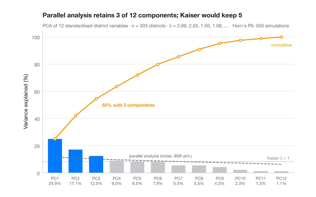
カリフォルニア州の 303 学区を記述するには何次元が必要か?成分ごとの分散と平行分析による基準。
factoextra::fviz_eig()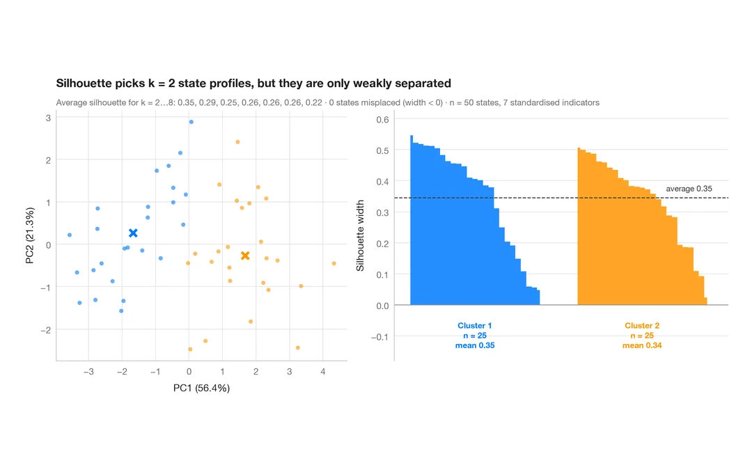
k-means のシルエットプロット
米国の州ははっきり異なる社会的プロファイルに分かれるか?k-means のクラスターとシルエット幅。
factoextra::fviz_silhouette()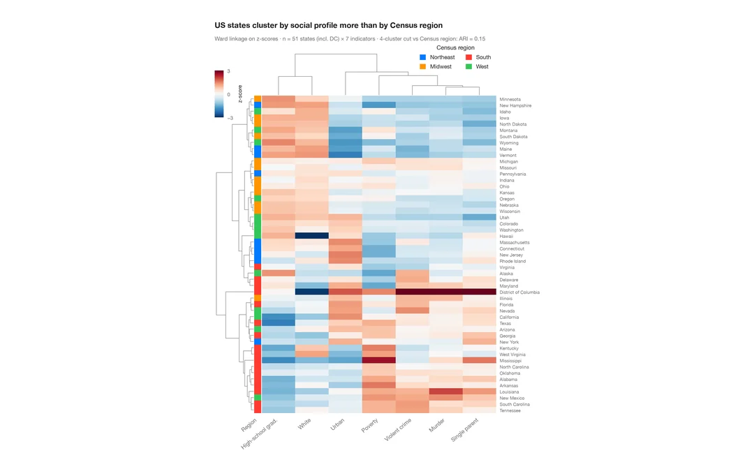
クラスター化ヒートマップ
米国各州の社会指標の z スコアのヒートマップ。行と列のデンドログラム、国勢調査地域のカラーバー付き。
pheatmap::pheatmap() / ComplexHeatmap::Heatmap()