Diverging Likert chart
Five-point Likert items as diverging stacked bars centred on the neutral answer.
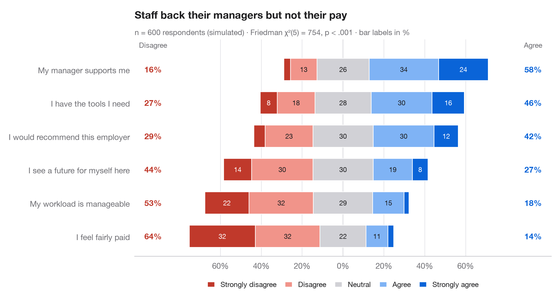
The Python counterpart of gglikert(). Each row is one survey item; the bar is
split into the five answer levels and shifted so that the neutral answer sits
astride zero: disagreement grows to the left, agreement to the right. Items are
sorted by total agreement, and the side columns give the total share who
disagree (left) and agree (right), so rows can be compared without reading segments.
Data are a seeded simulation of 600 employees answering six workplace statements.
Percentages come from pd.crosstab(normalize="index"); the subtitle reports a
Friedman test (scipy.stats.friedmanchisquare) asking whether the items
receive the same distribution of answers from the same respondents.
import matplotlib.pyplot as plt
import numpy as np
import pandas as pd
from scipy import stats

# Simulated survey: 600 respondents, 6 items, answers 1-5 driven by a shared latent mood
rng = np.random.default_rng(42)
items = {"My workload is manageable": -0.6, "I have the tools I need": 0.4,
         "My manager supports me": 0.8, "I feel fairly paid": -1.0,
         "I would recommend this employer": 0.2, "I see a future for myself here": -0.2}
mood = rng.normal(0, 0.8, 600)
answers = pd.DataFrame({item: np.digitize(shift + mood + rng.normal(0, 1, 600),
                                          [-1.6, -0.5, 0.5, 1.6]) + 1
                        for item, shift in items.items()})

levels = ["Strongly disagree", "Disagree", "Neutral", "Agree", "Strongly agree"]
colors = ["#C0392B", "#F1948A", "#D1D1D6", "#7FB3F5", "#0A64D8"]
pct = answers.melt().pipe(lambda d: pd.crosstab(d.variable, d.value, normalize="index") * 100)
pct["agree"], pct["disagree"] = pct[4] + pct[5], pct[1] + pct[2]
pct = pct.sort_values("agree")

# Friedman test: do the six items get the same answers from the same people?
fr = stats.friedmanchisquare(*[answers[c] for c in answers])

fig, ax = plt.subplots(figsize=(9.5, 5))
y = np.arange(len(pct))
left = -(pct[1] + pct[2] + pct[3] / 2)              # start so that neutral is centred on 0
for lev, (name, c) in enumerate(zip(levels, colors), start=1):
    ax.barh(y, pct[lev], left=left, color=c, height=0.66, label=name, edgecolor="white", lw=0.8)
    for yi, (l, w) in enumerate(zip(left, pct[lev])):
        if w >= 6:
            ax.text(l + w / 2, yi, f"{w:.0f}", ha="center", va="center", fontsize=8.5,
                    color="white" if lev in (1, 5) else "#1D1D1F")
    left = left + pct[lev]

# Totals on both sides
for yi, (d, a) in enumerate(zip(pct["disagree"], pct["agree"])):
    ax.text(-93, yi, f"{d:.0f}%", ha="center", va="center", fontsize=10, color="#C0392B", fontweight="semibold")
    ax.text(93, yi, f"{a:.0f}%", ha="center", va="center", fontsize=10, color="#0A64D8", fontweight="semibold")
ax.text(-93, len(pct) - 0.35, "Disagree", ha="center", fontsize=9, color="#6E6E73")
ax.text(93, len(pct) - 0.35, "Agree", ha="center", fontsize=9, color="#6E6E73")

ax.axvline(0, color="#3A3A3C", lw=0.8, zorder=0)
ax.spines["left"].set_visible(False)
ax.set_yticks(y, pct.index)
ax.set_xlim(-102, 102)
ax.set_ylim(-0.6, len(pct) - 0.1)
ax.set_xticks(range(-60, 61, 20), [f"{abs(t)}%" for t in range(-60, 61, 20)])
ax.grid(axis="x"); ax.grid(axis="y", visible=False)
ax.legend(ncols=5, loc="upper center", bbox_to_anchor=(0.5, -0.08), fontsize=9,
          handlelength=1, columnspacing=1.2)
ax.set_title("Staff back their managers but not their pay", pad=26)
ax.text(0, 1.02, f"n = {len(answers)} respondents (simulated) · Friedman χ²({answers.shape[1] - 1}) = "
        f"{fr.statistic:.0f}, p < .001 · bar labels in %", transform=ax.transAxes,
        fontsize=9.5, color="#6E6E73")
plt.show()
Figures use the optional PyStatlas style: add plt.style.use("pystatlas.mplstyle") to match the look exactly.
Data source
- Simulated data. Simulated data with a fixed random seed, created for this example.
No real respondents, documents or measurements: the numbers only illustrate how the chart and its statistics work.
The examples illustrate statistical methods. Their titles describe what each figure shows in these particular data — often a small, dated or partial sample — not the author's position on the substantive question. For interpretation, context and data quality, rely on the original sources cited here.
How to cite
PyStatlas is created and maintained by Thierry Warin. If it helped your work, please cite it.
Warin, T. (2026). Diverging Likert chart. In PyStatlas: A Python Gallery of Statistical Graphics for the Social Sciences. https://warint.github.io/pystatlas/proportions-surveys/likert-diverging/
@misc{warin2026statlas,
  author       = {Warin, Thierry},
  title        = {PyStatlas: A Python Gallery of Statistical Graphics for the Social Sciences},
  year         = {2026},
  howpublished = {\url{https://warint.github.io/pystatlas/}},
  note         = {Source code: https://github.com/warint/pystatlas}
}More in Proportions & surveys
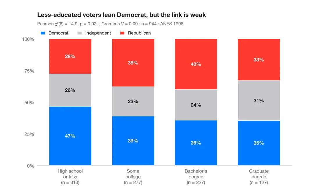
Stacked proportions by group
100% stacked bars with percentage labels, n per bar, chi-squared test and Cramér's V.
ggstatsplot::ggbarstats()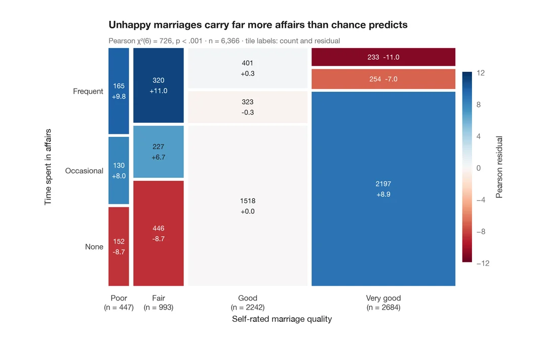
Mosaic plot with Pearson residuals
Tile areas proportional to cell counts, shaded by Pearson residuals from independence.
vcd::mosaic(shade = TRUE)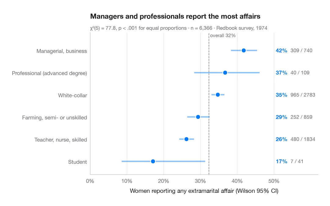
Proportions with confidence intervals
A sorted dot plot of group proportions with Wilson 95% confidence intervals.
ggstats::stat_prop() + geom_errorbar()