发散式 Likert 图
以中性回答为中心的发散堆叠条形图,展示五点 Likert 题项。
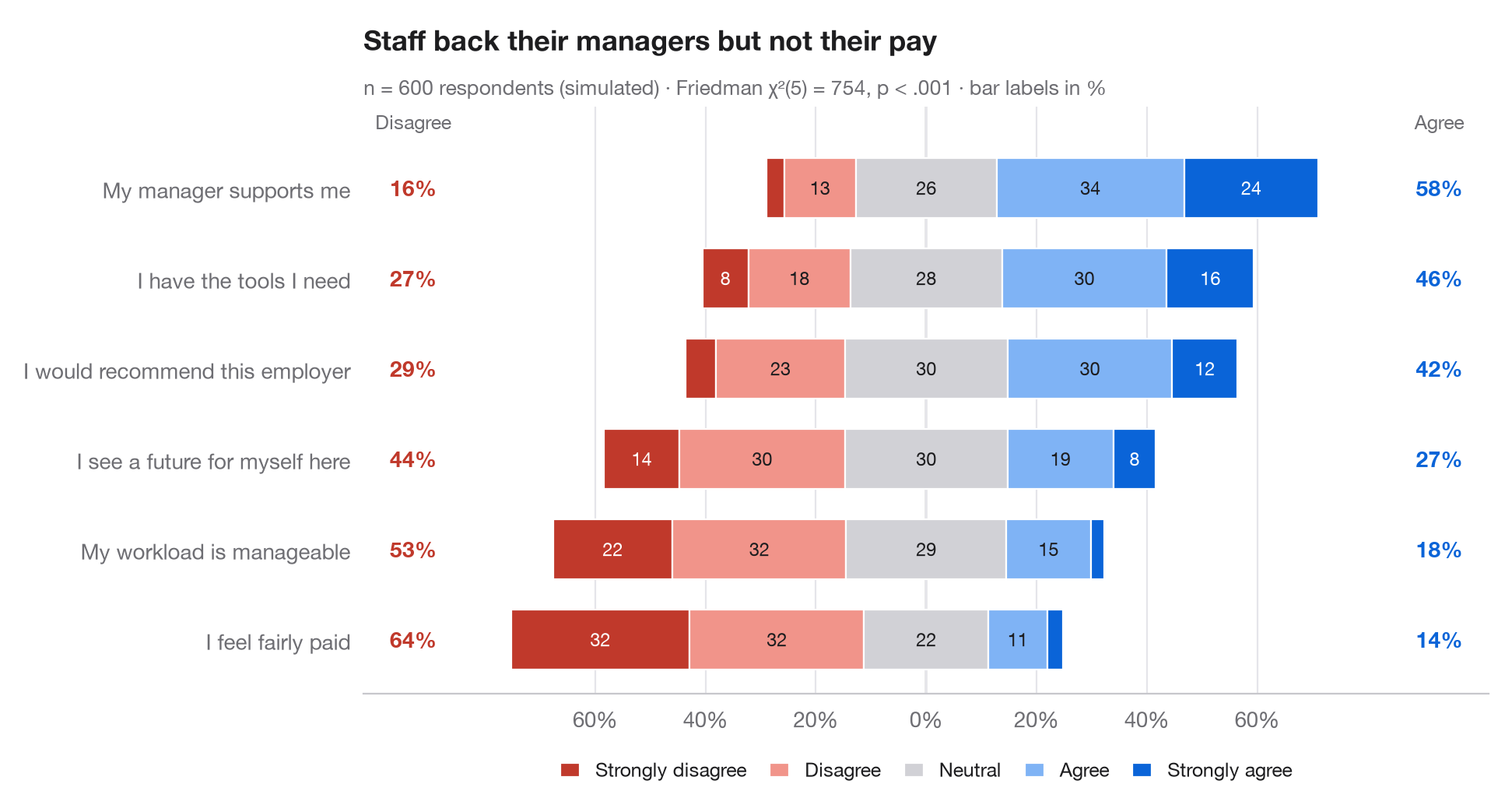
gglikert() 的 Python 版本。每一行是一道问卷题项;条形被分成五个回答等级,并经过平移,使中性回答横跨零点:不同意向左延伸,同意向右延伸。题项按总体同意程度排序,两侧的列分别给出不同意(左)和同意(右)的总比例,无需逐段阅读即可比较各行。
数据为设定了随机种子的模拟:600 名员工对六条职场陈述的回答。百分比由 pd.crosstab(normalize="index") 计算;副标题报告 Friedman 检验(scipy.stats.friedmanchisquare),检验同一批受访者对各题项的回答分布是否相同。
代码及图中文字均为英文。
import matplotlib.pyplot as plt
import numpy as np
import pandas as pd
from scipy import stats

# Simulated survey: 600 respondents, 6 items, answers 1-5 driven by a shared latent mood
rng = np.random.default_rng(42)
items = {"My workload is manageable": -0.6, "I have the tools I need": 0.4,
         "My manager supports me": 0.8, "I feel fairly paid": -1.0,
         "I would recommend this employer": 0.2, "I see a future for myself here": -0.2}
mood = rng.normal(0, 0.8, 600)
answers = pd.DataFrame({item: np.digitize(shift + mood + rng.normal(0, 1, 600),
                                          [-1.6, -0.5, 0.5, 1.6]) + 1
                        for item, shift in items.items()})

levels = ["Strongly disagree", "Disagree", "Neutral", "Agree", "Strongly agree"]
colors = ["#C0392B", "#F1948A", "#D1D1D6", "#7FB3F5", "#0A64D8"]
pct = answers.melt().pipe(lambda d: pd.crosstab(d.variable, d.value, normalize="index") * 100)
pct["agree"], pct["disagree"] = pct[4] + pct[5], pct[1] + pct[2]
pct = pct.sort_values("agree")

# Friedman test: do the six items get the same answers from the same people?
fr = stats.friedmanchisquare(*[answers[c] for c in answers])

fig, ax = plt.subplots(figsize=(9.5, 5))
y = np.arange(len(pct))
left = -(pct[1] + pct[2] + pct[3] / 2)              # start so that neutral is centred on 0
for lev, (name, c) in enumerate(zip(levels, colors), start=1):
    ax.barh(y, pct[lev], left=left, color=c, height=0.66, label=name, edgecolor="white", lw=0.8)
    for yi, (l, w) in enumerate(zip(left, pct[lev])):
        if w >= 6:
            ax.text(l + w / 2, yi, f"{w:.0f}", ha="center", va="center", fontsize=8.5,
                    color="white" if lev in (1, 5) else "#1D1D1F")
    left = left + pct[lev]

# Totals on both sides
for yi, (d, a) in enumerate(zip(pct["disagree"], pct["agree"])):
    ax.text(-93, yi, f"{d:.0f}%", ha="center", va="center", fontsize=10, color="#C0392B", fontweight="semibold")
    ax.text(93, yi, f"{a:.0f}%", ha="center", va="center", fontsize=10, color="#0A64D8", fontweight="semibold")
ax.text(-93, len(pct) - 0.35, "Disagree", ha="center", fontsize=9, color="#6E6E73")
ax.text(93, len(pct) - 0.35, "Agree", ha="center", fontsize=9, color="#6E6E73")

ax.axvline(0, color="#3A3A3C", lw=0.8, zorder=0)
ax.spines["left"].set_visible(False)
ax.set_yticks(y, pct.index)
ax.set_xlim(-102, 102)
ax.set_ylim(-0.6, len(pct) - 0.1)
ax.set_xticks(range(-60, 61, 20), [f"{abs(t)}%" for t in range(-60, 61, 20)])
ax.grid(axis="x"); ax.grid(axis="y", visible=False)
ax.legend(ncols=5, loc="upper center", bbox_to_anchor=(0.5, -0.08), fontsize=9,
          handlelength=1, columnspacing=1.2)
ax.set_title("Staff back their managers but not their pay", pad=26)
ax.text(0, 1.02, f"n = {len(answers)} respondents (simulated) · Friedman χ²({answers.shape[1] - 1}) = "
        f"{fr.statistic:.0f}, p < .001 · bar labels in %", transform=ax.transAxes,
        fontsize=9.5, color="#6E6E73")
plt.show()
图表使用了可选的 PyStatlas 样式:添加 plt.style.use("pystatlas.mplstyle") 即可完全还原其外观。
数据来源
- Simulated data. Simulated data with a fixed random seed, created for this example.
No real respondents, documents or measurements: the numbers only illustrate how the chart and its statistics work.
这些示例用于说明统计方法。图表标题描述的是该图在这些特定数据中呈现的内容——这些数据往往样本较小、年代较早或并不完整——而不是作者对实质问题的立场。关于解释、背景和数据质量,请以此处引用的原始来源为准。
如何引用
PyStatlas 由 Thierry Warin 创建并维护。如果它对你的工作有所帮助,敬请引用。
Warin, T. (2026). Diverging Likert chart. In PyStatlas: A Python Gallery of Statistical Graphics for the Social Sciences. https://warint.github.io/pystatlas/proportions-surveys/likert-diverging/
@misc{warin2026statlas,
  author       = {Warin, Thierry},
  title        = {PyStatlas: A Python Gallery of Statistical Graphics for the Social Sciences},
  year         = {2026},
  howpublished = {\url{https://warint.github.io/pystatlas/}},
  note         = {Source code: https://github.com/warint/pystatlas}
}