Stacked proportions by group

Warin, Thierry

100% stacked bars with percentage labels, n per bar, chi-squared test and Cramér's V.

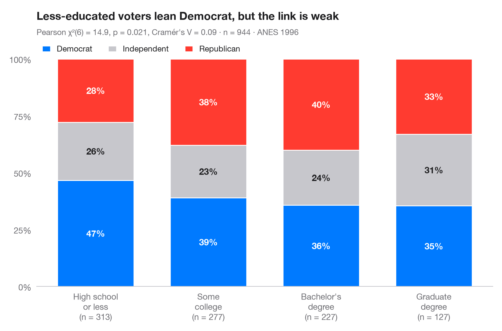
The Python counterpart of ggbarstats(). Each bar is one group rescaled to 100%, so the segments show the conditional distribution of the outcome within the group; the labels are row percentages and the number under each bar is the group size. The subtitle reports Pearson's χ² test of independence and Cramér's V, the effect size that rescales χ² to the 0–1 range.

Data are the 1996 American National Election Study bundled with statsmodels (sm.datasets.anes96): party identification of 944 voters by education. The test comes from scipy.stats.chi2_contingency and V from scipy.stats.contingency.association.

stacked-proportions.py · 43 lines

Download GitHub

import matplotlib.pyplot as plt
import numpy as np
import pandas as pd
import statsmodels.api as sm
from scipy import stats
from scipy.stats.contingency import association

# Data: 1996 ANES — party identification (7-point scale) by education (7 levels)
df = sm.datasets.anes96.load_pandas().data
df["party"] = pd.cut(df.PID, [-1, 1, 4, 6], labels=["Democrat", "Independent", "Republican"])
df["education"] = pd.cut(df.educ, [0, 3, 5, 6, 7],
                         labels=["High school\nor less", "Some\ncollege", "Bachelor's\ndegree", "Graduate\ndegree"])

table = pd.crosstab(df.education, df.party)
pct = table.div(table.sum(axis=1), axis=0) * 100

# Pearson chi-squared test of independence + Cramér's V
chi2, p, dof, _ = stats.chi2_contingency(table, correction=False)
v = association(table.to_numpy(), method="cramer")

fig, ax = plt.subplots(figsize=(8, 5.2))
colors = ["#007AFF", "#C7C7CC", "#FF3B30"]
x = np.arange(len(pct))
bottom = np.zeros(len(pct))
for party, c in zip(pct.columns, colors):
    ax.bar(x, pct[party], bottom=bottom, color=c, width=0.68, label=party, edgecolor="white", lw=1)
    for xi, (b, h) in enumerate(zip(bottom, pct[party])):
        ax.text(xi, b + h / 2, f"{h:.0f}%", ha="center", va="center", fontsize=10.5,
                fontweight="semibold", color="#1D1D1F" if c == "#C7C7CC" else "white")
    bottom += pct[party].to_numpy()

ax.set_xticks(x, [f"{g}\n(n = {n})" for g, n in zip(pct.index, table.sum(axis=1))])
ax.set_yticks(range(0, 101, 25), [f"{t}%" for t in range(0, 101, 25)])
ax.set_ylim(0, 100)
ax.grid(False)
ax.spines["left"].set_visible(False)
ax.legend(ncols=3, loc="lower left", bbox_to_anchor=(0, 1.0), fontsize=9.5,
          handlelength=1, borderaxespad=0.3)
ax.set_title("Less-educated voters lean Democrat, but the link is weak", pad=46)
ax.text(0, 1.105, f"Pearson χ²({dof}) = {chi2:.1f}, p = {p:.3f}, Cramér's V = {v:.2f} · "
        f"n = {table.to_numpy().sum()} · ANES 1996", transform=ax.transAxes,
        fontsize=9.5, color="#6E6E73")
plt.show()

Figures use the optional PyStatlas style: add plt.style.use("pystatlas.mplstyle") to match the look exactly.

Data source

American National Election Study, 1996. Rosenstone, S. J., Kinder, D. R., Miller, W. E., & the National Election Studies. (2016). ANES 1996 Time Series Study (ICPSR 6896; Version 6) [Data set]. Inter-university Consortium for Political and Social Research. https://doi.org/10.3886/ICPSR06896.v6
Subset of 944 respondents distributed with statsmodels (sm.datasets.anes96); public domain.

The examples illustrate statistical methods. Their titles describe what each figure shows in these particular data — often a small, dated or partial sample — not the author's position on the substantive question. For interpretation, context and data quality, rely on the original sources cited here.

How to cite

PyStatlas is created and maintained by Thierry Warin. If it helped your work, please cite it.

Warin, T. (2026). Stacked proportions by group. In PyStatlas: A Python Gallery of Statistical Graphics for the Social Sciences. https://warint.github.io/pystatlas/proportions-surveys/stacked-proportions/

@misc{warin2026statlas,
  author       = {Warin, Thierry},
  title        = {PyStatlas: A Python Gallery of Statistical Graphics for the Social Sciences},
  year         = {2026},
  howpublished = {\url{https://warint.github.io/pystatlas/}},
  note         = {Source code: https://github.com/warint/pystatlas}
}

More in Proportions & surveys

Proportions & surveys

Diverging Likert chart

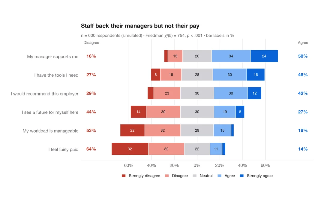
Five-point Likert items as diverging stacked bars centred on the neutral answer.

ggstats::gglikert()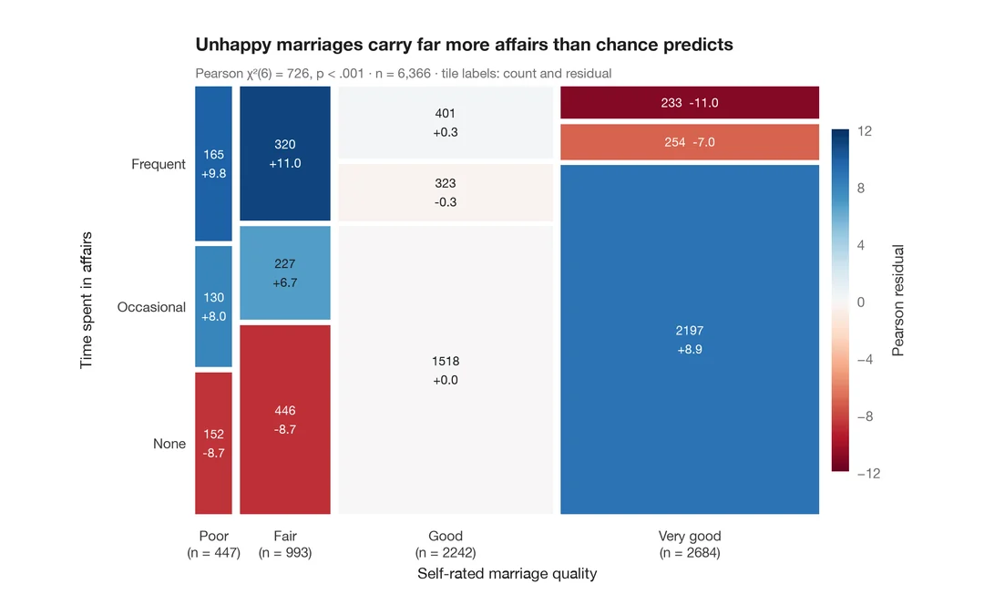

Proportions & surveys

Mosaic plot with Pearson residuals

Tile areas proportional to cell counts, shaded by Pearson residuals from independence.

vcd::mosaic(shade = TRUE)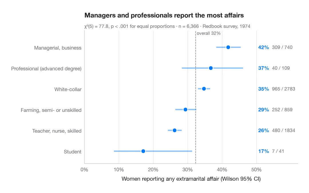

Proportions & surveys

Proportions with confidence intervals

A sorted dot plot of group proportions with Wilson 95% confidence intervals.

ggstats::stat_prop() + geom_errorbar()